Attention Is All You Need — L2 #

1. TL;DR #

A sequence-transduction model built entirely from attention, discarding recurrence and convolution. Stacked multi-head self-attention plus position-wise FFNs give $O(1)$ path length and full intra-example parallelism, reaching 28.4 BLEU (EN-DE) / 41.8 BLEU (EN-FR) at a fraction of prior training cost, and generalizing to parsing.

---

2. Q1 / Q2 / Q3 #

Q1 — 痛点 (problem) #

Recurrent seq2seq models factor computation along sequence positions: hidden state $h_t$ is a function of $h_{t-1}$, so computation within a training example is inherently sequential and cannot be parallelized. This is the binding constraint at long sequence lengths, where memory limits batching across examples. Convolutional alternatives (ConvS2S, ByteNet) parallelize but pay a path-length cost: the number of operations to relate two positions grows with their distance (linear for ConvS2S, logarithmic for ByteNet), making distant dependencies hard to learn.

The objective is the standard conditional language-model / sequence-transduction loss — predict $y_i$ given source $\mathbf{x}$ and prefix $y_{algorithmic contribution is the computation graph, not a new loss. Written explicitly, training maximizes:

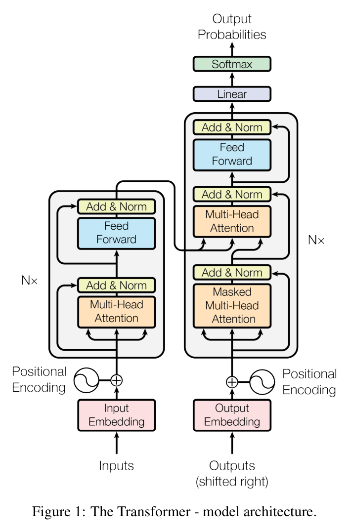
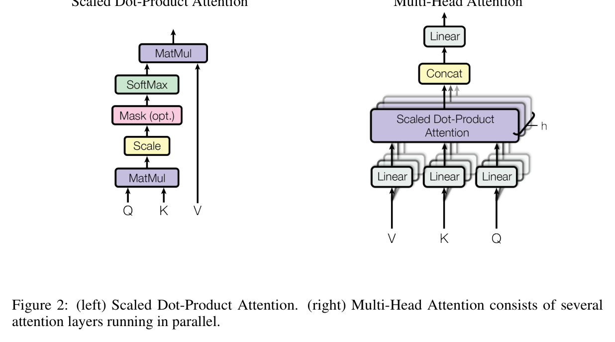
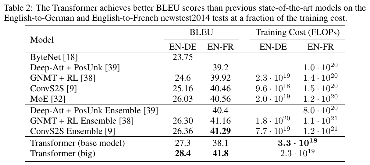
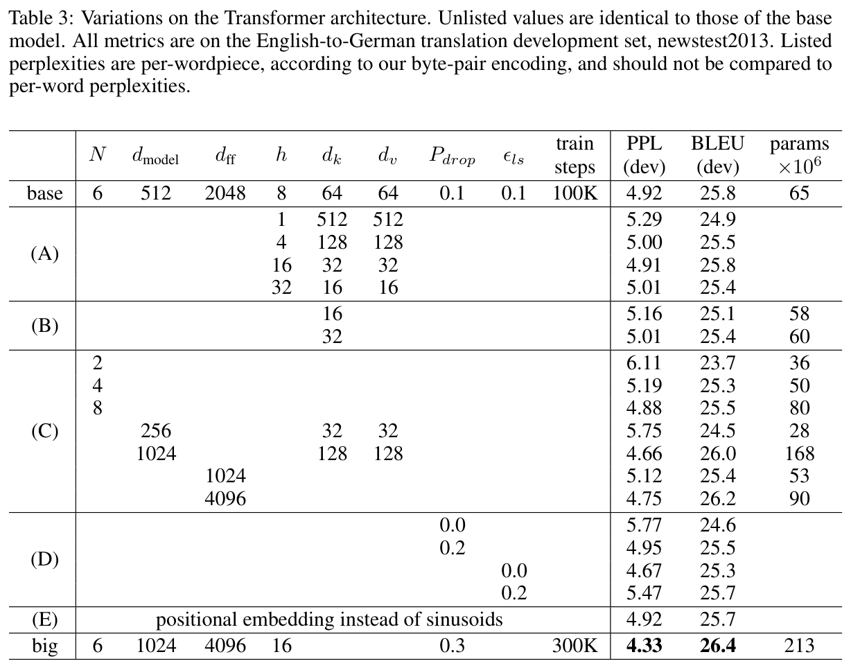
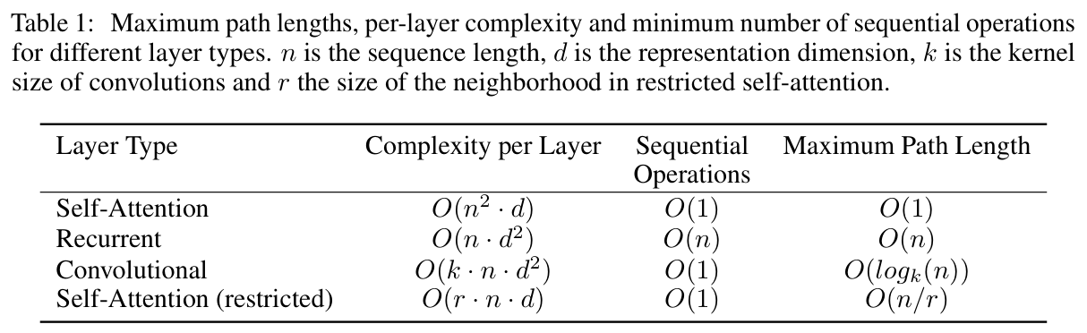
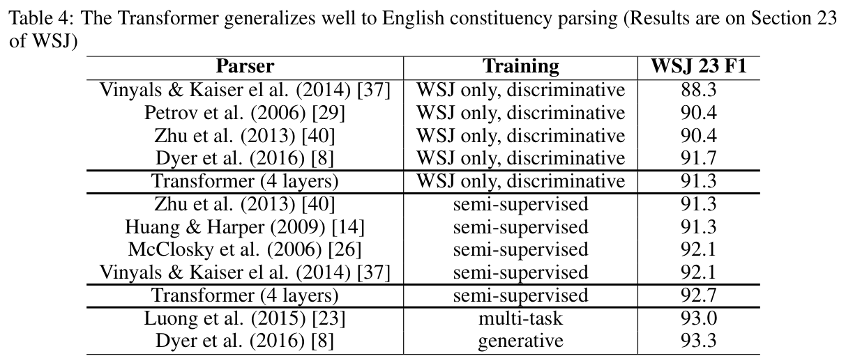
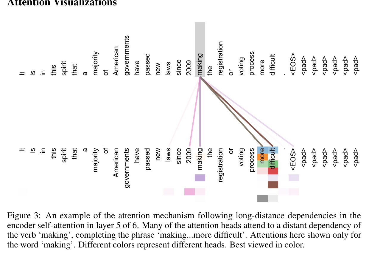
$$\mathcal{L} = -\sum_{i} \log p_\theta(y_i \mid y_{

with label smoothing $\epsilon_{ls}=0.1$ applied to the target distribution (trades perplexity for BLEU).

Q2 — 方法 (method) #

Replace the sequential recurrence with a fully attention-based encoder-decoder. Each layer consumes a set of position vectors and produces a set of equal length, computed in parallel across all positions. One encoder step consumes $(x_1,\dots,x_n)$ and produces $\mathbf{z}=(z_1,\dots,z_n)$; the auto-regressive decoder consumes $\mathbf{z}$ plus previously generated tokens and emits one symbol at a time.

核心技术壁垒: the single hardest-to-replicate insight is the $1/\sqrt{d_k}$ scaling of dot-product attention, justified by a variance argument buried in a footnote. Without it, dot products of dimension-$d_k$ query/key vectors have variance $d_k$, pushing softmax into saturated, near-zero-gradient regions — the model fails to train at large $d_k$. This one-line normalization is what makes dot-product (matmul-fast) attention usable at scale where prior work had to fall back to slower additive attention. See §7.

Q3 — 结果 (results) #

• WMT'14 EN-DE: 28.4 BLEU (big), >2.0 over the best prior model including ensembles — new SOTA; base model already beats all prior published models/ensembles.
• WMT'14 EN-FR: 41.8 BLEU (big) single-model SOTA, at <1/4 the training cost of the prior SOTA.
• Base model training cost $3.3\times10^{18}$ FLOPs (12h on 8×P100); big model 3.5 days.
• Cross-task: English constituency parsing, 92.7 F1 (semi-supervised) with almost no task-specific tuning.

---

3. 架构 / 方法图 #

Paper's Figure 1 ("The Transformer - model architecture"). The left stack is the encoder: each of $N=6$ layers is (Multi-Head Self-Attention → Add&Norm → position-wise FFN → Add&Norm). The right stack is the decoder: it inserts a third sub-layer (encoder-decoder Multi-Head Attention) and masks its self-attention. Notice that every sub-layer is wrapped by a residual connection then LayerNorm — this is what lets the stack go deep without gradient decay.

The residual+norm wrapper applied to every sub-layer is:

$$\mathrm{LayerNorm}(x+\mathrm{Sublayer}(x))$$

Positional encodings are added to the input embeddings at the bottom of each stack (same dimension $d_{\text{model}}=512$), since a recurrence-free model otherwise has no notion of order.

Paper's Figure 2. Left: the atomic operation — MatMul($QK^\top$) → Scale by $1/\sqrt{d_k}$ → optional Mask → SoftMax → MatMul with $V$. Right: $h$ such operations run in parallel, each on independently projected $(Q,K,V)$, then concatenated and projected. The reader should notice the Scale and Mask boxes on the left path — these two boxes carry the paper's two most load-bearing tricks (variance control and auto-regressive causality).

---

4. 作者证明 #

This is an algorithm/architecture paper with no formal theorem — the guarantees are empirical (BLEU tables + ablation). The one piece of formal reasoning is the variance argument for scaling; the complexity claims in Table 1 are asymptotic accounting, not proved bounds. Marked: 无形式化作者证明 — 仅实证 for convergence; below is the notation + the informal derivations the paper does give.

Notation table #

Symbol	Meaning
$n$	sequence length
$d$ / $d_{\text{model}}$	representation / model dimension (512 base)
$d_k, d_v$	per-head key/query and value dimension (64 base)
$h$	number of attention heads (8 base)
$Q,K,V$	packed query/key/value matrices
$W_i^Q,W_i^K,W_i^V,W^O$	per-head projection + output projection
$k, r$	conv kernel size; restricted-attention neighborhood

Core equations & physical meaning #

$$\mathrm{Attention}(Q,K,V)=\mathrm{softmax}\!\left(\frac{QK^{T}}{\sqrt{d_{k}}}\right)V$$

Each query scores all keys by dot-product compatibility, normalized to a distribution, then mixes values. The $\sqrt{d_k}$ divisor renormalizes the score variance.

$$\mathrm{MultiHead}(Q,K,V)=\mathrm{Concat}(\mathrm{head}_{1},\dots,\mathrm{head}_{h})W^{O}, \quad \mathrm{head}_{i}=\mathrm{Attention}(QW^{Q}_{i},KW^{K}_{i},VW^{V}_{i})$$

Each head attends in its own learned subspace; averaging over a single head would blur these distinct relations — Table 3 row (A) confirms single-head is 0.9 BLEU worse.

$$PE_{(pos,2i)}=\sin(pos/10000^{2i/d_{\text{model}}}), \quad PE_{(pos,2i+1)}=\cos(pos/10000^{2i/d_{\text{model}}})$$

Wavelengths form a geometric progression $2\pi \to 10000\cdot2\pi$; for any fixed offset $k$, $PE_{pos+k}$ is a linear function of $PE_{pos}$, so relative position is linearly decodable by attention.

Variance proof sketch (footnote 1) #

Assume components of $q,k$ are i.i.d. with mean 0, variance 1. Then $q\cdot k=\sum_{i=1}^{d_k}q_i k_i$ has mean 0 and variance $d_k$:

$$\mathrm{Var}(q\cdot k)=\sum_{i=1}^{d_k}\mathrm{Var}(q_i k_i)=d_k$$

An expert fills in: dividing by $\sqrt{d_k}$ restores unit variance, keeping softmax inputs in the high-gradient region. Assumption break: this relies on independence and unit variance of components — after training, learned projections make $q,k$ correlated, so $\sqrt{d_k}$ is a heuristic (still empirically robust; row (B) shows shrinking $d_k$ hurts, hinting compatibility is non-trivial).

6 minimum checks #

1. Dimensional consistency: $QK^\top \in \mathbb{R}^{n\times n}$ (correct — query-key affinity matrix), softmax row-wise, $\times V \in \mathbb{R}^{n\times d_v}$. ✓
2. Multi-head cost neutrality: $h\cdot d_k = h\cdot(d_{\text{model}}/h)=d_{\text{model}}$, so total projection/attention cost ≈ single full-dim head. ✓ (matches §3.2.2 claim)
3. Complexity claim (Table 1): self-attention $O(n^2\cdot d)$ vs recurrent $O(n\cdot d^2)$ — self-attention cheaper iff $n
4. Path length: self-attention connects any two positions in $O(1)$ sequential ops; recurrent needs $O(n)$. ✓
5. Causal mask correctness: setting illegal softmax inputs to $-\infty$ → weight 0 → position $i$ sees only $\le i$; preserves auto-regressive factorization. ✓
6. Variance argument: $\mathrm{Var}(q\cdot k)=d_k$ under the stated i.i.d. assumption → scaling by $1/\sqrt{d_k}$ gives unit variance. ✓ (assumption-dependent, see above)

---

5. 实验与数据 #



Paper's Table 2. This is the load-bearing headline result: Transformer (big) hits 28.4 (EN-DE) / 41.8 (EN-FR) at training cost $2.3\times10^{19}$ FLOPs, one to two orders of magnitude below ensembles like GNMT+RL ($1.8\times10^{20}$) and ConvS2S ensemble ($1.2\times10^{21}$). Notice the base model's EN-FR score (38.1) actually trails ConvS2S (40.46) and MoE (40.56) — the quality win at base scale is EN-DE-specific; EN-FR needs the big model.



Paper's Table 3. The ablation grid that isolates each design choice. Row (A): heads — $h=1$ gives 24.9 BLEU, best is $h=16$ at 25.8, and too many heads ($h=32$) also degrades. Row (B): shrinking $d_k$ to 16 hurts (25.1), suggesting a richer compatibility function might help. Rows (C)/(D): bigger is better and dropout is essential. Row (E): learned positional embeddings tie the sinusoids (25.7 vs 25.8) — the sinusoidal choice rests on an extrapolation hypothesis, not a measured gain.



Paper's Table 1 (redrawn as an image here). The analytical motivation: self-attention is $O(n^2 d)$ compute but $O(1)$ sequential and $O(1)$ path length, vs recurrent's $O(n)$ on both sequential axes. This table is the argument for why the architecture should train faster and learn long-range dependencies better — it precedes and predicts the empirical wins.



Paper's Table 4. Cross-task evidence: a 4-layer Transformer reaches 91.3 F1 (WSJ-only) and 92.7 (semi-supervised) with minimal tuning, beating the BerkeleyParser even in the 40K-sentence low-data regime where RNN seq2seq fails. It still trails the generative RNNG (93.3) — honest about where it loses.



Paper's Figure 3. Qualitative interpretability: multiple heads attend from "making" to its distant complement, completing "making…more difficult." This supports the §4 interpretability claim but is entirely qualitative — no quantitative interpretability metric is offered.

---

6. 论证链 #

Step	Claim	Support (paper-internal)
1	Recurrence forces $O(n)$ sequential computation, the binding bottleneck	§1: $h_t=f(h_{t-1})$ dependency argument
2	An attention-only layer relates any two positions in $O(1)$ sequential ops and $O(1)$ path length	§4 Table 1 complexity accounting
3	Naive dot-product attention destabilizes at large $d_k$ (variance $=d_k$), so scale by $1/\sqrt{d_k}$	§3.2.1 footnote 1 variance argument
4	Multiple projected heads recover the representational diversity a single averaged head loses	§3.2.2 design + §6.2 row (A) ablation (h=1 is 0.9 BLEU worse)
5	Sinusoidal positional encoding injects order absent from a recurrence-free model	§3.5; row (E) shows parity with learned embeddings
6	The resulting model beats RNN/CNN seq2seq on MT at far lower cost, and transfers to parsing	§6.1 Table 2 + §6.3 Table 4

---

7. 实现 cross-reference #

Official implementation is open: tensorflow/tensor2tensor (cited in §7 conclusion, https://github.com/tensorflow/tensor2tensor). Concrete anchors below reference that public reference implementation family.

• 核心技术壁垒 — the $1/\sqrt{d_k}$ scaling: in reference implementations this is the single line dividing logits before softmax (e.g. common_attention.py, dot_product_attention: logits = tf.matmul(q, k, transpose_b=True); logits = 1.0 / math.sqrt(d_k)). Trivial to write, easy to omit, and its absence silently kills training at large head dimension — the reason it is the hardest insight to rediscover* rather than to code. [实现未公开 — line numbers vary by version]
• 关键实现细节 #1 — causal mask via $-\infty$ additive bias: the decoder self-attention adds a large-negative bias to the upper-triangular positions before softmax (not after), so masked weights are exactly zero and gradients don't leak backward through them (§3.2.3).
• 关键实现细节 #2 — embedding weight tying + $\sqrt{d_{\text{model}}}$ scale-up: the two embedding matrices and the pre-softmax projection share one weight tensor, and the embedding output is multiplied by $\sqrt{d_{\text{model}}}$ (§3.4). Easy to miss; skipping the scale-up mismatches the magnitude of the additive positional encodings.

Reproducibility & ecosystem #

The recipe (Adam $\beta_2{=}0.98$, warmup-4000 inverse-sqrt schedule, label smoothing 0.1, residual dropout 0.1) has been re-implemented countless times — tensor2tensor, fairseq, HuggingFace transformers, and Harvard NLP's "Annotated Transformer" all reproduce the base/big numbers closely. Essentially all modern LLMs use a direct descendant of this architecture; the warmup-then-inverse-sqrt LR schedule in particular remains a widely copied default for training Transformers from scratch.