Language Models are Few-Shot Learners (GPT-3)
Language Models are Few-Shot Learners (GPT-3) — L2 #
1. TL;DR #
Scaling a plain GPT-2-style autoregressive decoder to 175B parameters makes
task-agnostic in-context learning work: with no gradient updates, GPT-3
learns tasks purely from prompt demonstrations, sometimes matching fine-tuned
SOTA. The load-bearing finding is that the zero→few-shot gap widens with
scale — larger models are disproportionately better meta-learners.
2. Q1 / Q2 / Q3 #
Q1 — 痛点 (What problem?) #
The dominant pretrain-then-finetune paradigm is task-agnostic in architecture
but not in data: every new task needs thousands to hundreds of thousands
of labeled examples (§1). Three concrete pains motivate the paper:
- Practicality: collecting a large supervised set per task limits where
- Spurious correlations: fine-tuning on a narrow distribution lets a model
- Human contrast: humans learn a new language task from a directive or a
- In-context learning scales: the zero/one/few-shot gap grows with model
- Sometimes matches SOTA fine-tuning: TriviaQA few-shot 71.2% (closed-book
- Emergent on-the-fly reasoning: 100% on 2-digit addition, 98.9% on 2-digit
- Human-indistinguishable text: humans detect 175B-generated ~200-word news
- Persistent weaknesses: NLI (ANLI, RTE), WiC (49.4% = chance), and
- FFN width: $d_{\mathrm{ff}} = 4 \cdot d_{\mathrm{model}}$ — fixes MLP expansion
- Answer-context normalization (ARC/OpenBookQA/RACE):
- Empirical scaling law (from Fig 3.1): $L = 2.57 \cdot C^{-0.048}$ — validation
- Compute accounting: forward pass costs 2 flops/active-param/token (1 add + 1
- Param-breakdown / capacity: 175B model = 96 layers ×
- Compute cross-check: $6 \times 1.746\times10^{11} \times 3\times10^{11}
- Scaling-law fit: authors fit kaplan2020scaling's power law; Fig 3.1's
- KV bytes/token (175B, fp16): $2 \times n_{\mathrm{layers}} \times
- Data budget: Table 2.2 epochs are self-consistent — 300B training tokens
- Overfitting check: Fig 4.1 shows train/val gap grows only minimally with
- The alternating dense / locally-banded sparse attention (child2019generating)
- Sequence packing without cross-document masking: multiple documents are
- Minimum serving footprint: 175B in fp16 ≈ 350 GB just for weights ⇒
- KV bytes/token: ~4.7 MB/token (fp16, dense-attn layers, from §4 check 4);
- Amortized cost: once trained, generating 100 pages costs ~0.4 kW-hr /
- Saturation/inversion: at what scale does the widening few-shot gap stop
- Objective ceiling: the equal-weight next-token objective is ungrounded and
- Hardware affinity: GPT-3 predates FP8/FP4 — would a dense-MHA 175B benefit
LMs can be used.
exploit dataset artifacts, so nominally human-level benchmark scores may
exaggerate true task ability (§1 para 4, citing hendrycks2020pretrained,
mccoy2019right, niven2019probing).
handful of examples; NLP systems cannot.
Prior in-context learning (GPT-2) showed the idea was possible but far behind
fine-tuning (e.g. 4% on Natural Questions), so meta-learning was not yet viable.
Q2 — 方法 (What method?) #
Test one hypothesis: *since log-loss follows a smooth power law with scale
(kaplan2020scaling), in-context learning ability should also grow with scale.*
Concretely — train 8 dense decoder-only Transformers (125M→175B), identical
to GPT-2 (modified init, pre-norm, reversible BPE) except for **alternating
dense and locally-banded sparse attention** layers borrowed from the Sparse
Transformer (child2019generating). Evaluate every model in three settings —
zero-shot (instruction only), one-shot (one demo), few-shot (K≈10–100 demos) —
with zero gradient updates; the model is conditioned purely by text in a
2048-token context window (§2).
核心技术壁垒: the replicable-in-principle-but-not-in-practice insight is not the architecture (it is deliberately a vanilla GPT-2) but the industrial-scale data + compute + parallelism pipeline that trains a stable 175B dense model on 300B quality-weighted tokens across depth- and width-partitioned V100s. Everything downstream (emergent arithmetic, the widening few-shot gap) is an emergent consequence of executing that pipeline at a scale nobody had reached, not of any algorithmic novelty. See §7.
Q3 — 结果 (What result?) #
size (§1 para 16; aggregate curves).
SOTA), LAMBADA few-shot 86.4% (+18%), CoQA few-shot 85.0 F1 (near human),
PTB zero-shot perplexity 20.5 (−15 vs SOTA).
subtraction, with a memorization spot-check finding <1% of problems in
training.
at ~52% (chance), even spending more time as models grow.
comparison/re-reading reading-comprehension tasks (QuAC, RACE).
3. 架构 / 方法图 #
GPT-3 is a decoder-only autoregressive Transformer reusing the GPT-2
architecture wholesale. The distinguishing design axis is *scale + evaluation
protocol*, not module invention. The paper's central conceptual figure is the
meta-learning "inner-loop / outer-loop" picture:
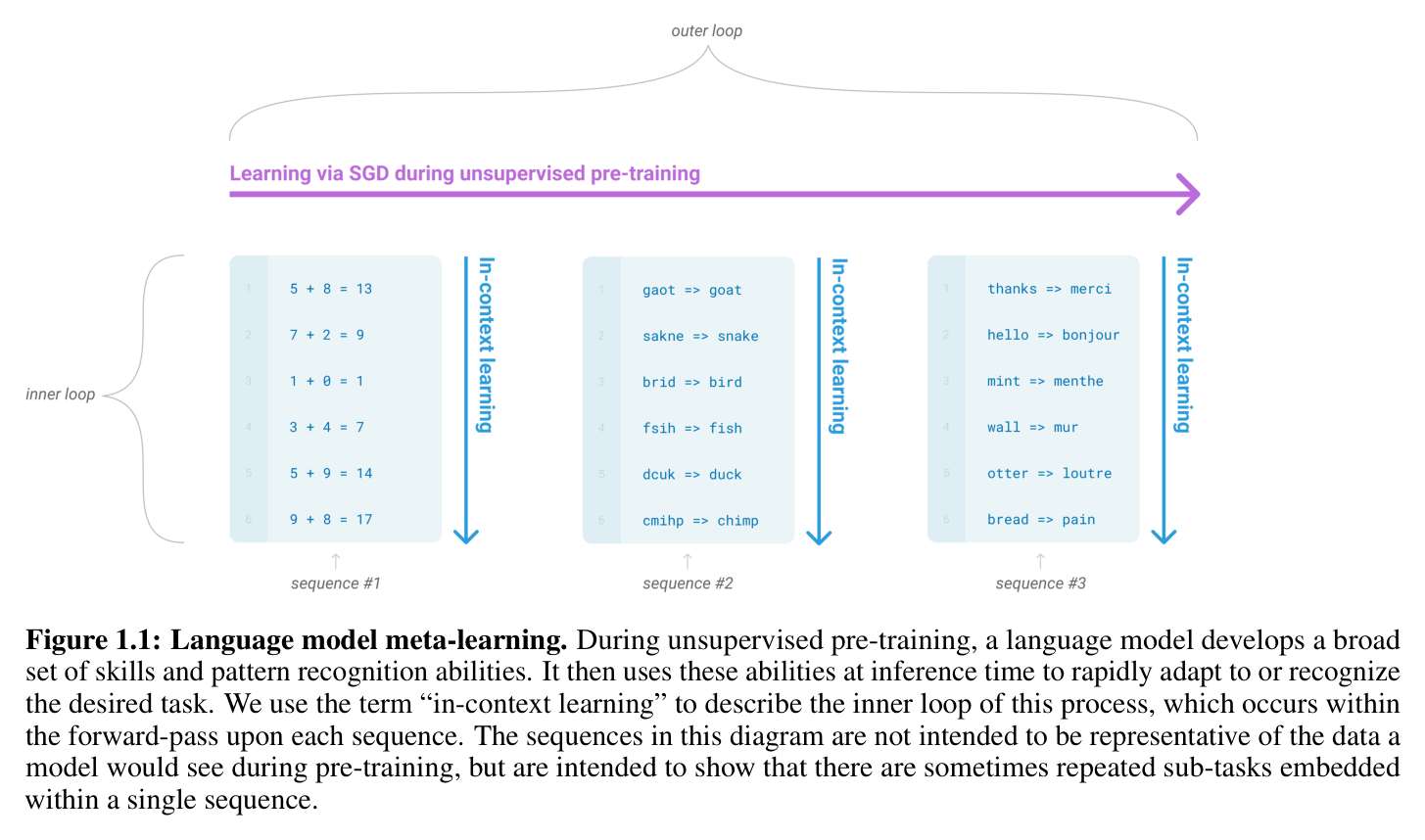
*Paper's Figure 1.1, verbatim (caption: "Language model meta-learning. During
unsupervised pre-training, a language model develops a broad set of skills and
pattern recognition abilities. It then uses these abilities at inference time
to rapidly adapt to or recognize the desired task...").*
This figure encodes the paper's whole thesis: the outer loop is ordinary
SGD pretraining; the inner loop ("in-context learning") is a *single
forward pass* over a sequence that happens to contain repeated sub-tasks
(arithmetic 5+8=13, transliteration gaot ⇒ goat, translation
thanks ⇒ merci). No weights change in the inner loop — adaptation is pure
conditioning. This is why the four evaluation settings below are all
"forward-pass only".
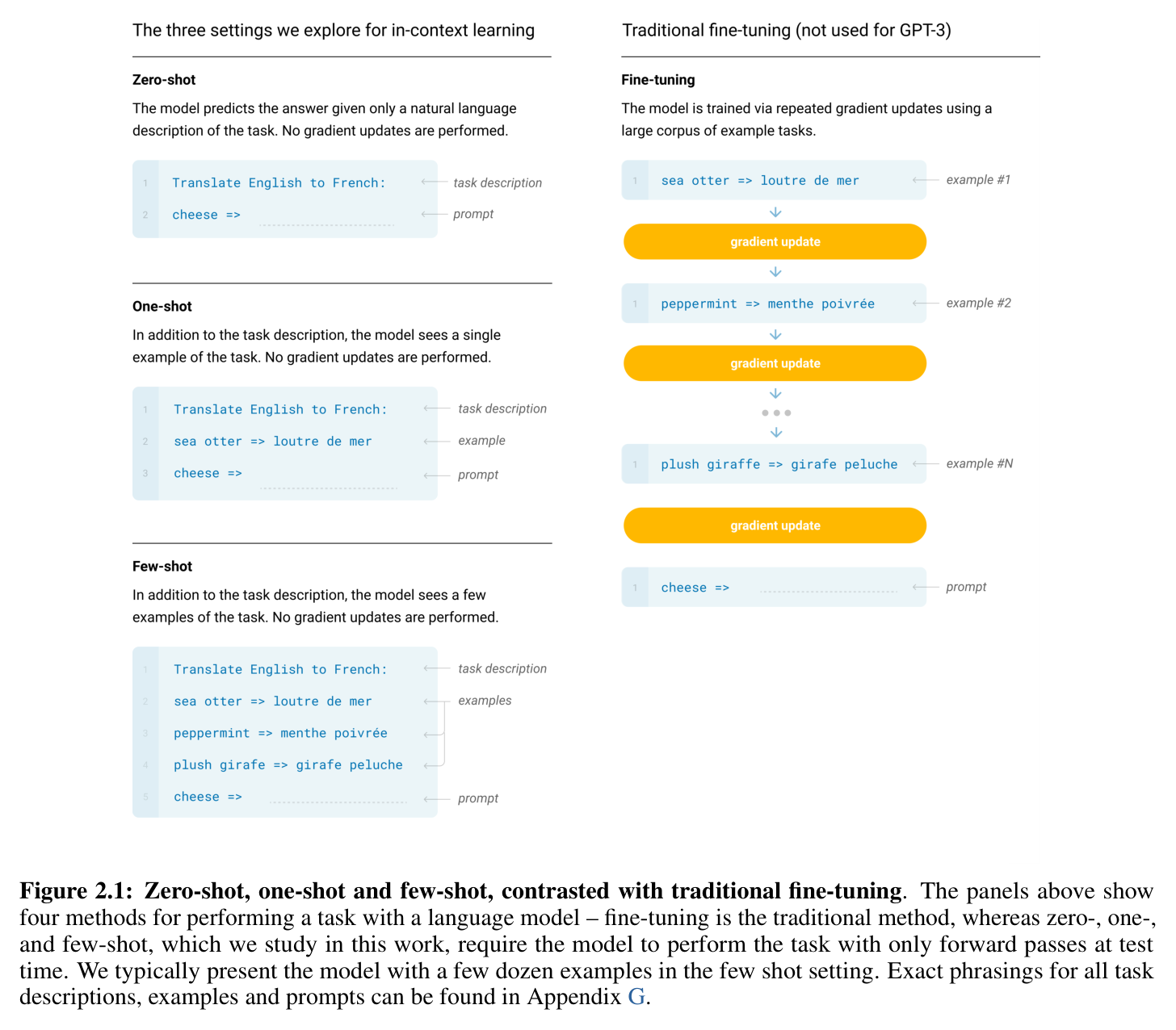
*Paper's Figure 2.1, verbatim (caption: "Zero-shot, one-shot and few-shot,
contrasted with traditional fine-tuning...").* The right column shows
fine-tuning inserting a gradient update after every example; the three left
panels (studied here) only stack more demonstrations into the prompt before the
final cheese => query. The reader should notice that few-shot's "learning"
never touches parameters — it is entirely in the context.
Concrete architecture family #
The 8-model family fixes d_ff = 4·d_model and scales only depth/width:
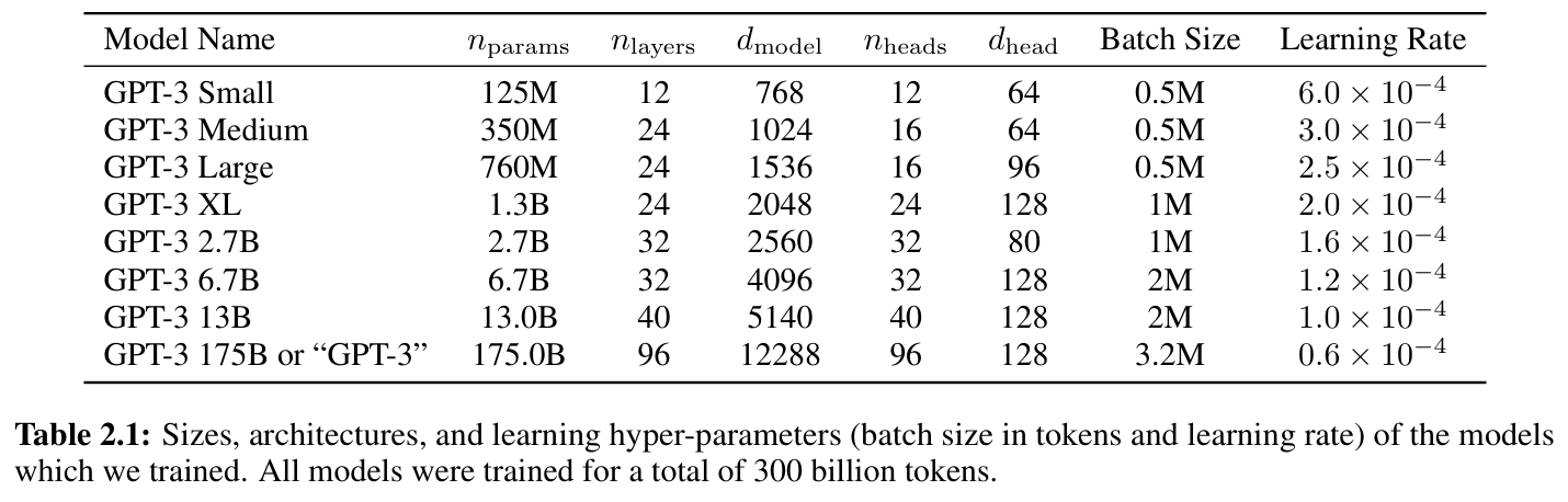
*Paper's Table 2.1, verbatim (caption: "Sizes, architectures, and learning
hyper-parameters ... All models were trained for a total of 300 billion
tokens").* Notice the co-scaling regularities: batch size grows
(0.5M→3.2M tokens) while LR shrinks ($6.0\times10^{-4}$→$0.6\times10^{-4}$),
guided by gradient-noise-scale measurement; the 175B model is 96 layers ×
$d_{\mathrm{model}}=12288$ × 96 heads of dim 128, $n_{\mathrm{ctx}}=2048$.
Top-level data flow (GPT-2-identical) #
Per-block detail (pre-norm, MHA, GeLU MLP) #
Attention variant: standard MHA (no GQA/MQA/MLA), learned absolute
position embeddings (wpe, not RoPE), plus the paper's one twist — alternating
dense and locally-banded sparse attention across layers
(child2019generating) to cut the $O(n^2)$ cost at $n_{\mathrm{ctx}}=2048$.
KV shape per layer = [batch, n_heads, seq, head_dim=128].
FFN variant: dense GeLU MLP with 4× expansion — **no MoE, no gating,
no shared experts**.
Norm/position: pre-norm LayerNorm (GPT-2 layout) + a final ln_f;
absolute learned positions capped at 2048.
4. 作者证明 #
There is no formal theorem; GPT-3's "proof" is the analytical
compute-accounting model (App D) plus the empirical power-law extrapolation
(Fig 3.1). The load-bearing equations are notation for evaluation and compute,
and the fitted scaling curve.
Notation table #
| Symbol | Meaning | Source |
|---|---|---|
| $d_{\mathrm{model}}$ | residual/bottleneck width | Table 2.1 |
| $d_{\mathrm{ff}}$ | FFN hidden width, fixed $=4\,d_{\mathrm{model}}$ | §2.1 |
| $n_{\mathrm{ctx}}$ | context window $=2048$ | §2.1 |
| $K$ | number of in-context demonstrations | §2.4 |
| $C$ | training compute (PF-days) | Fig 3.1 |
| $L$ | cross-entropy validation loss | Fig 3.1 |
| $\alpha$ | Pareto shape for CC quality resampling $=9$ | App A |
Load-bearing equations & physical meaning #
so only depth/width vary across the 8 models.
$\frac{P(\mathrm{completion}\mid\mathrm{context})}{P(\mathrm{completion}\mid\mathrm{answer\_context})}$
— divides out a completion's prior likelihood so answers are scored on
task-relevant evidence, not surface frequency.
loss as a power law in compute; the tiny exponent $-0.048$ means loss falls
slowly but predictably across ~10 orders of magnitude of compute.
multiply), the backward pass adds a 3× multiplier, and
$1\text{ PF-day}=8.64\times10^{19}$ flops (App D).
6 minimum checks #
$d_{\mathrm{model}}=12288$. Per-layer dense params ≈ attention
($4\,d^2 = 4\cdot12288^2 \approx 6.0\times10^8$) + MLP
($8\,d^2 = 8\cdot12288^2 \approx 1.2\times10^9$) $\approx 1.8\times10^9$;
× 96 layers ≈ $1.74\times10^{11}$ — matches the reported 175B
(embeddings excluded), consistent with App D's 174,600 M.
\approx 3.14\times10^{23}$ flops $= 3.14\times10^{23}/8.64\times10^{19}
\approx 3.6\times10^{3}$ PF-days — matches App D's 3.64E+03.
$L=2.57\,C^{-0.048}$ is reproduced by their own curve and holds "2 more
orders of magnitude" with only slight deviation.
n_{\mathrm{heads}} \times d_{\mathrm{head}} \times 2\text{ B} =
2\cdot96\cdot96\cdot128\cdot2 \approx 4.7\text{ MB/token}$ (dense-attn
layers); banded-sparse layers reduce effective attended length, not stored
KV — a first-principles number the paper itself does not tabulate.
with CC weighted 60% ⇒ 0.44 epochs of a 410B-token corpus
($0.6\cdot300/410 \approx 0.44$); Wikipedia 3% ⇒
$0.03\cdot300/3 \approx 3.0$ (≈ reported 3.4 with rounding).
size and time, supporting the claim that loss gains are not corpus
memorization (corroborated by §4 contamination analysis and the arithmetic
spot-check).
5. 实验与数据 #
Training recipe itemization (equal weight to architecture) #
| Stage | Goal | Data (tokens + mix) | LR schedule | Context | Techniques |
|---|---|---|---|---|---|
| Pre-training (single stage) | Learn broad skills for in-context use | 300B tokens; CC 60% / WebText2 22% / Books1 8% / Books2 8% / Wikipedia 3% (quality-weighted, non-proportional) | Adam ($\beta_1{=}0.9,\beta_2{=}0.95,\epsilon{=}10^{-8}$); cosine decay to 10% over 260B tokens; linear warmup over first 375M tokens | 2048; sequences packed, docs delimited by EOT, no special masking | grad-norm clip 1.0; weight decay 0.1; batch ramp 32k→full over first 4–12B tokens; depth+width model parallel on V100 |
| Mid-training / annealing | [论文未披露] | [论文未披露] | [论文未披露] | [论文未披露] | [论文未披露] |
| SFT | [论文未披露 — GPT-3 is base-model only] | [论文未披露] | [论文未披露] | [论文未披露] | [论文未披露] |
| Post-training (DPO/RLHF/…) | [论文未披露 — explicitly left to future work, §2/§5] | [论文未披露] | [论文未披露] | [论文未披露] | [论文未披露] |
| Quantization-aware training | N/A — not discussed | — | — | — | — |
Single hardest-to-replicate training trick: the **quality-weighted,
non-proportional sampling** of the corpus (CC and Books2 sampled <1 epoch,
Wikipedia/WebText2 2–3 epochs) combined with the Pareto-based CC quality
resampler ($\alpha=9$, App A). The paper openly trades "a small amount of
overfitting for higher quality" — the exact classifier, feature set, and
threshold that make a 175B dense model stable on this mix are the secret sauce.
Smooth scaling with compute #
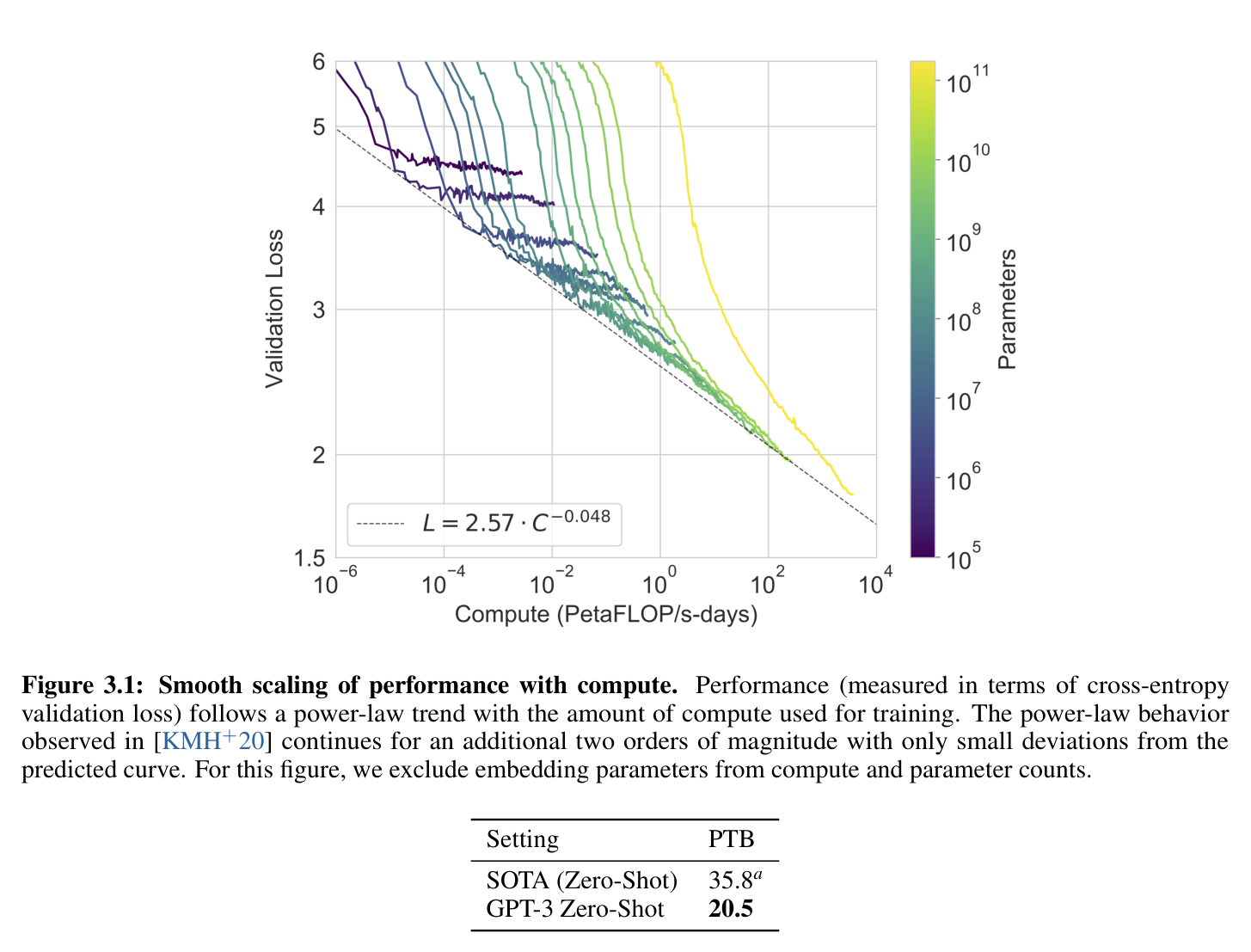
*Paper's Figure 3.1, verbatim (caption: "Smooth scaling of performance with
compute. Performance (measured in terms of cross-entropy validation loss)
follows a power-law trend ... continues for an additional two orders of
magnitude").* The dashed fit $L = 2.57\cdot C^{-0.048}$ (color = param count,
$10^5$→$10^{11}$) is the empirical backbone of the whole scaling bet: loss keeps
falling predictably, so the authors argue downstream ability should too. The
reader should notice how little the largest (yellow) curves deviate from the
extrapolated line.
Training curves: gap is difficulty, not overfitting #
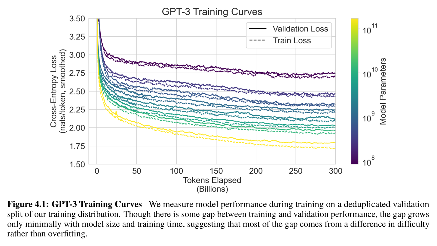
*Paper's Figure 4.1, verbatim (caption: "GPT-3 Training Curves ... the gap
grows only minimally with model size and training time, suggesting that most of
the gap comes from a difference in difficulty rather than overfitting").* Solid
= validation, dashed = train. Because the two nearly overlap even for the
175B (yellow) run over 300B tokens, the paper can argue that improvements in
cross-entropy reflect genuine generalization — directly supporting the §4
claim that benchmark contamination has little effect.
Bias audit (societal results) #
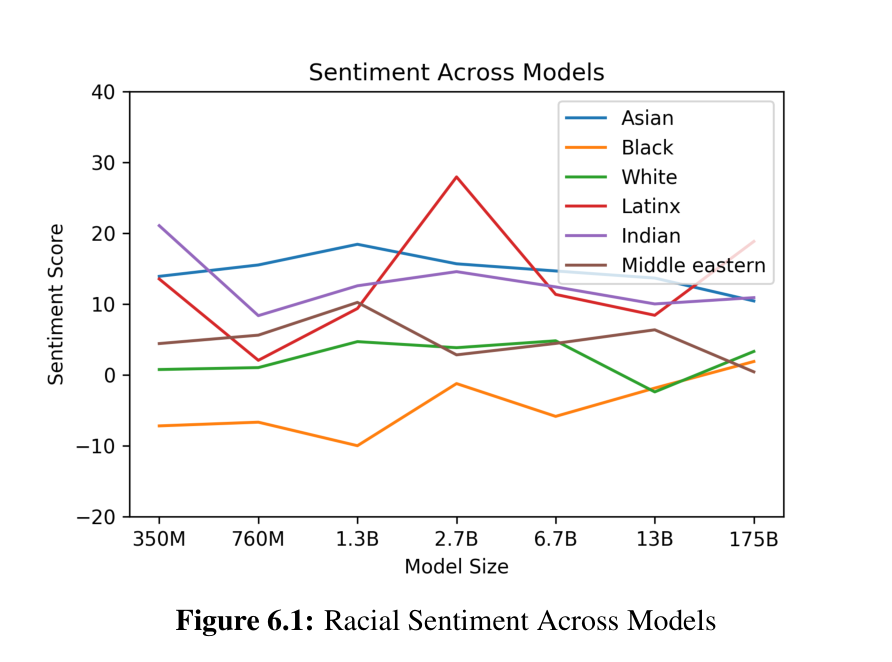
Paper's Figure 6.1, verbatim (caption: "Racial Sentiment Across Models").
"Asian" ranks highest in 3/7 models and "Black" lowest in 5/7; the reader
should notice the gaps narrow only marginally with scale — scaling does not
自动 remove internet-scale bias.
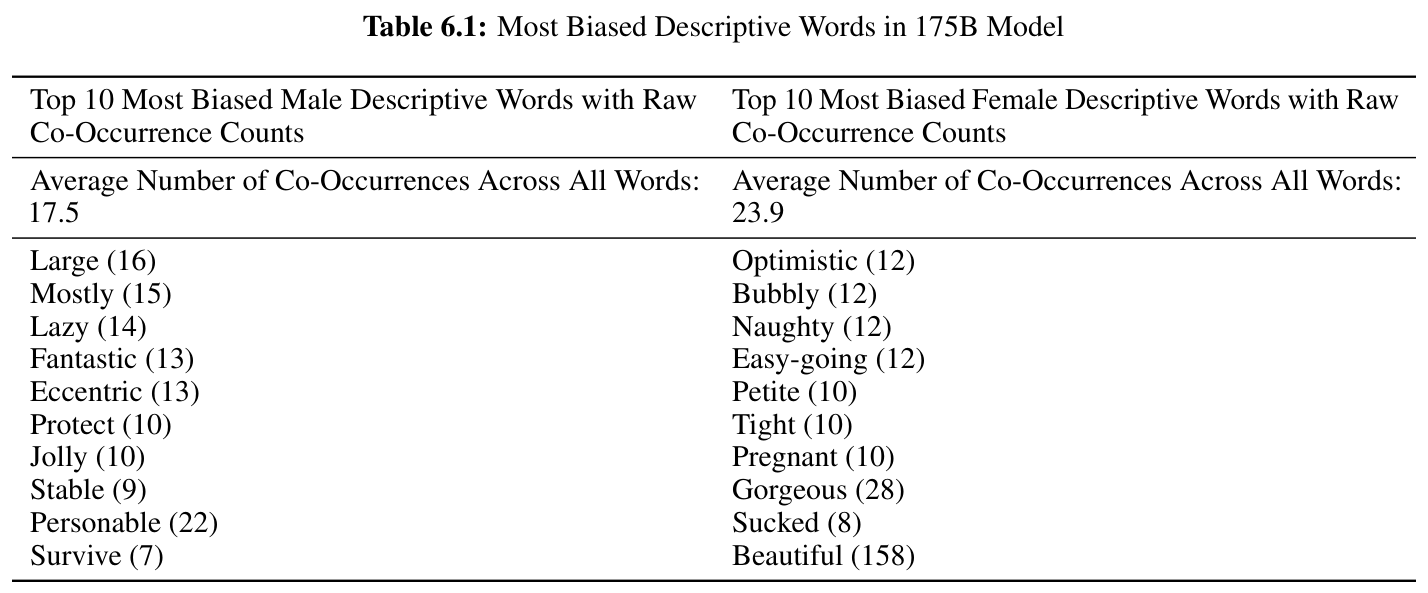
*Paper's Table 6.1, verbatim (caption: "Most Biased Descriptive Words in 175B
Model").* Female-associated words skew appearance-oriented ("Beautiful" 158,
"Gorgeous" 28) versus a broader male spectrum; the raw counts make the
gender-occupation bias (avg log-odds $-1.11$ neutral, $-2.14$ "competent")
concrete rather than anecdotal.
Headline benchmark numbers (175B) #
| Task | Metric | FT-SOTA | GPT-3 0S | 1S | FS |
|---|---|---|---|---|---|
| PTB | ppl | 35.8 | 20.5 | — | — |
| LAMBADA | acc | 68.0 | 76.2 | 72.5 | 86.4 |
| TriviaQA | acc | 68.0 (RAG) | 64.3 | 68.0 | 71.2 |
| CoQA | F1 | 90.7 | 81.5 | 84.0 | 85.0 |
| SuperGLUE | avg | 89.0 | 58.2 | 68.9 | 71.8 (test) |
| WiC | acc | 76.1 | — | — | 49.4 (chance) |
| ANLI R3 | acc | 48.3 | 34.5 | 35.1 | 40.2 |
| 2-digit add | acc | — | 76.9 | 99.6 | 100.0 |
6. 论证链 #
| # | Step | Evidence (paper-internal) |
|---|---|---|
| 1 | Fine-tuning needs per-task labeled data and can exploit spurious correlations | §1 paras 2–4 |
| 2 | Prior LM validation loss follows a smooth power law with scale | Fig 3.1 ($L=2.57\,C^{-0.048}$); kaplan2020scaling |
| 3 | ∴ If loss predicts downstream ability, scaling should improve in-context learning | §1 para 8 (stated hypothesis) |
| 4 | Train 8 dense decoder models 125M→175B, evaluate 0/1/few-shot with no gradients | §2.1 Table 2.1; §2.4 protocol |
| 5 | Loss keeps falling on-trend and train≈val, so gains are generalization not memorization | Fig 3.1 (extrapolation), Fig 4.1 (gap stable) |
| 6 | Downstream few-shot scores rise with size, and the 0→few-shot gap widens with size | §1 para 16; aggregate + per-task scale plots |
| 7 | ∴ Larger models are better meta-learners; few-shot sometimes matches FT-SOTA | TriviaQA 71.2, LAMBADA 86.4, CoQA 85.0 |
| 8 | But some abilities (NLI, WiC, comparison/re-reading tasks) resist scaling | §3.7 WiC 49.4, §3.8 ANLI, §5 unidirectionality argument |
7. 实现 cross-reference #
GPT-3's weights and training code are [实现未公开]. However, GPT-3's
architecture is GPT-2 verbatim (§2.1), so the runnable inference structure is
faithfully reproduced by the vLLM GPT-2 model. All dims below are config-driven
(the 175B config populates hidden_size=12288, num_hidden_layers=96,
num_attention_heads=96 per Table 2.1).
Fused QKV + output projection, head_dim = hidden/heads:
        self.c_attn = QKVParallelLinear(
            self.hidden_size,
            self.head_dim,
            total_num_heads,
            bias=True,
4× FFN expansion (the d_ff = 4·d_model rule) with GeLU:
        inner_dim = config.n_inner if config.n_inner is not None else 4 * hidden_size

        self.ln_1 = nn.LayerNorm(hidden_size, eps=config.layer_norm_epsilon)
Pre-norm block with two residual adds (A2 diagram source of truth):
        residual = hidden_states
        hidden_states = self.ln_1(hidden_states)
        attn_output = self.attn(hidden_states=hidden_states)
        # residual connection
        hidden_states = attn_output + residual
Learned absolute positions added to token embeddings (not RoPE):
            if inputs_embeds is None:
                inputs_embeds = self.embed_input_ids(input_ids)
            position_embeds = self.wpe(position_ids)
            hidden_states = inputs_embeds + position_embeds
关键实现细节 (easy-to-miss tricks):
is GPT-3's only architectural deviation from GPT-2 — the stock vLLM GPT-2
above is dense-only, so a faithful 175B replica must interleave banded
masks layer-by-layer, a detail absent from any public config.
concatenated into each 2048-token sequence, delimited only by an EOT token
with no special attention mask (App B) — cheap to implement but silently
lets attention leak across doc boundaries, an accepted trade-off for speed.
§8 Serving deployment considerations #
≥5–8× 80 GB GPUs before KV cache; the paper notes inference is "expensive and
inconvenient" and floats distillation (§5, §6.3).
the banded-sparse layers cut attended length but not stored KV, so long
contexts are memory-bound.
a few cents (§6.3) — training is thousands of PF-days but inference is cheap.
§9 Open questions (LLM-specific) #
paying off, and do comparison tasks (WiC/ANLI) ever cross chance without a
bidirectional objective (§5 conjecture)?
prediction-not-action; does the recipe transfer to vision/audio, or does it
need a learned/RL objective (§5 para 3)?
from low-precision inference, or does dense attention at 2048 ctx stay
memory-bound regardless? (paper does not address quantization.)
Appendix: 模型架构图 #
代码来源:https://github.com/vllm-project/vllm/blob/main/vllm/model_executor/models/gpt2.py (GPT-3 复用 GPT-2 架构,§2.1;维度取自 Table 2.1 的 175B 配置)
A1 — Top-Level #
No MTP head — GPT-3 is single-token autoregressive.
A2 — Block (pre-norm, standard residual) #
A3 — 主 Attention 变体 (MHA) #
A4 — 辅 Attention 变体 #
N/A — 模型仅使用单一 MHA(层间在 dense 与 locally-banded sparse 掩码之间交替,
但仍是同一 MHA 模块,无第二种 attention 类型)。
A5 — 选择/索引机制 #
N/A — 模型为 dense FFN,无 MoE routing / indexer / gating。
A6 — 残差/连接机制 #
N/A — 标准 pre-norm 残差(见 A2),无 mHC / Highway / DenseNet 式连接。
代码-图对照表 #
| 代码构件 | 对应图 | 关键实现细节 |
|---|---|---|
GPT2Model.wte + wpe (gpt2.py:199,205) | A1 | token + 学习式绝对位置相加;无 RoPE |
make_layers(num_hidden_layers, GPT2Block) (gpt2.py:206) | A1/A2 | 175B ⇒ 96 层;论文额外要求 dense/banded-sparse 交替(vLLM 默认 dense-only,差异见 §7) |
GPT2Block.forward (gpt2.py:171-182) | A2 | pre-norm,两处标准残差加 |
GPT2Attention.c_attn / c_proj (gpt2.py:80-102) | A3 | 融合 QKV,head_dim = hidden/heads = 128 |
GPT2MLP (gpt2.py:125-139) | — | inner_dim = 4·hidden 即 $d_{ff}=4d_{model}$,GeLU |
tie_weights(wte) (gpt2.py:289) | A1 | lm_head 与词嵌入权重共享 |