DistServe: Disaggregating Prefill and Decoding for Goodput-optimized Large Language Model Serving
DistServe — L2 distillation #
1. TL;DR #
DistServe splits LLM inference so prefill and decoding run on separate GPU pools, killing phase interference and letting each phase pick its own parallelism. A goodput-optimal placement search plus NVLINK-affinity KV transfer yields up to 7.4× higher request rate or 12.6× tighter SLO at >90% attainment.
2. Q1 / Q2 / Q3 #
Q1 — 痛点 (pain point). Existing serving systems colocate prefill and decoding on the same GPUs and batch both across requests to maximize aggregate throughput. This creates two coupled failures. First, prefill-decoding interference: a prefill step is compute-heavy and long, so when batched with decoding steps it stalls them (inflating TPOT), while adding decoding tokens to a prefill batch inflates TTFT. Second, resource + parallelism coupling: prefill wants intra-op parallelism to shrink execution time for tight TTFT, decoding wants large batches + a different parallelism plan for TPOT — colocation forces one shared plan tuned to the harder SLO, causing over-provisioning. The system optimizes throughput (tokens/s) but the real cost metric is per-GPU goodput — requests/s served within SLO per GPU.
Q2 — 方法 (method). Physically disaggregate the two phases onto separate "instances" (a unit owning one complete copy of weights). A prefill instance computes only the first token, then hands its KV cache to a decoding instance. Because the phases are decoupled, DistServe (a) co-optimizes GPU count + parallelism (intra-op TP / inter-op PP) per phase using a simulator-driven placement search, (b) replicates to hit the traffic rate, and (c) places segments bandwidth-aware so KV transfer rides NVLINK rather than the slow cross-node link.
核心技术壁垒 (the single hardest-to-replicate insight): the instance-segment colocation placement algorithm (Algorithm 2). The non-obvious observation is that KV-cache transfer happens only between corresponding inter-op stages of the prefill and decoding instances. By grouping layers into inter-op stages and forcing the same-stage prefill and decoding segments onto one physical node, all KV transfer stays on intra-node NVLINK — even a large model that cannot fit two full replicas in one 8-GPU node still transfers over NVLINK. This is what drops KV transfer to <0.1% of latency on a 25 Gbps cross-node testbed, and it is co-optimized jointly with the parallelism search rather than bolted on.
Q3 — 结果 (result). Against vLLM: 2.0–4.6× higher rate (chatbot), 5.7× (code completion), 4.3× (summarization) and up to 12.6× tighter SLO. Against DeepSpeed-MII (chunked-prefill): 1.6–7.4× higher rate. KV transfer <0.1% of total latency for OPT-175B; >95% of requests see <30 ms transfer. Ablation shows disaggregation — not parallelism tuning — is the load-bearing gain ("vLLM++" best-search ≈ plain vLLM). Placement search runs in minutes and is model-size-independent.
3. 架构 / 方法图 #
The motivation figure quantifies the "free lunch" of separation on a single 13B model / A100:
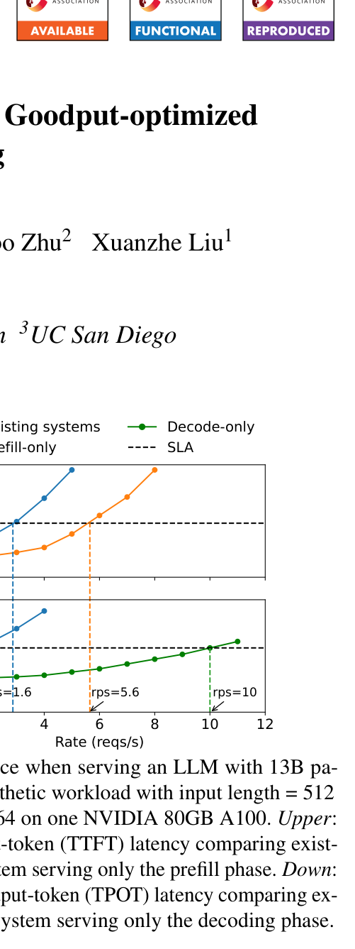
Paper's Figure 1: Upper = P90 TTFT for existing (colocated) systems vs a prefill-only system; Down = P90 TPOT for existing vs a decoding-only system, both vs request rate. Reading off the knees: colocated goodput is ~1.6 rps, but a prefill-only GPU sustains 5.6 rps and a decoding-only GPU 10 rps — so a 2-prefill + 1-decode split delivers 10 rps overall (3.3 rps/GPU), 2.1× the colocated system, with no new kernels, just reallocation.
The runtime lifecycle — arrival → centralized controller → prefill instance → KV pull → decoding instance — is shown here:
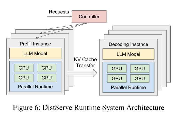
Paper's Figure 6: DistServe Runtime System Architecture. The scheduler is a centralized controller running plain FCFS: each request is dispatched to the prefill instance with the shortest queue, then to the least-loaded decoding instance. The KV/memory manager is separated from the scheduler and uses a pull discipline — decoding instances fetch KV from prefill instances on demand, using the prefill instance's HBM as a queuing buffer to absorb burstiness. Transport is asynchronous CudaMemcpy on NVLINK intra-node and NCCL cross-node.
The request lifecycle and the segment-colocation transport constraint can be seen structurally as:
The scheduling granularity is per-request for dispatch, but batch formation is token-count-driven: prefill batches are packed to a total sequence length near the compute-saturation threshold $L_m$, and decoding batches are packed to a max batch size (also named $L_m$ for the decode side) to keep execution time balanced across the pipeline and reduce bubbles.
4. 作者证明 #
This is a framework paper with a formal performance model (§3.1 M/D/1 queue + Appendix A latency model). Notation and checks below.
Notation table.
| Symbol | Meaning |
|---|---|
| $D$ | per-request prefill execution time (constant under uniform prompt length) |
| $R$ | Poisson arrival rate |
| $RD$ | utilization; stability requires $RD<1$ |
| $D_s$ | request-level latency under a given parallelism |
| $D_m$ | slowest-stage service time (inter-op) |
| $K$ | intra-op speedup coefficient, $1 |
| $h,n,s,m$ | hidden size, #heads, head size ($h=ns$), FFN intermediate size |
| $B,t,t_2$ | batch size, total tokens $t=\sum l_i$, squared-length sum $t_2=\sum l_i^2$ |
| $C_1..C_5$ | profiled latency constants |
Prefill single-device TTFT (M/D/1). Because one request saturates the GPU, requests are served FCFS without batching, giving a deterministic-service M/D/1 queue:
$$Avg\_TTFT = D + \frac{RD^2}{2(1-RD)}$$
Physical meaning: first term is raw execution, second is queuing delay that diverges as $RD\to1$.
Inter-op (2-way pipeline). With $D\approx D_s\approx 2D_m$ (inter-layer activation transfer is negligible), the bottleneck stage services at rate $1/D_m$:
$$Avg\_TTFT_{inter} = D_s + \frac{RD_m^2}{2(1-RD_m)} = D + \frac{RD^2}{4(2-RD)}$$
Intra-op (2-way tensor). Execution time drops to $D_s=D/K$ but sublinearly ($K<2$) due to communication:
$$Avg\_TTFT_{intra} = \frac{D}{K} + \frac{RD^2}{2K(K-RD)}$$
Prefill latency model (Appendix A.2), compute-bound GEMM + memory-bound attention:
$$T_{Prefill} = C_1\cdot(4th^2 + 2thm) + C_2\cdot\frac{3ht_2}{b} + C_3$$
Decoding latency model (Appendix A.3), both terms memory-bound:
$$T_{Decoding} = C_4\cdot(4h^2 + 2hm) + C_5\cdot 3ht$$
Six minimum checks:
- Why
min/sumstructure — the goodput objective is a min. Overall goodput is limited by the slower of the two phases; the placement replicates $n=\lceil R/config_p.goodput\rceil$ prefill and $m=\lceil R/config_d.goodput\rceil$ decoding instances, so each phase is provisioned to its own rate ceiling — the min over phases determines when SLO breaks. - Why divide by $K$, not by 2, in Eq.3. Intra-op cannot achieve perfect 2× speedup because of collective-communication overhead, so effective service rate is $K/D$ ($1
- Interior vs boundary optimum (monotonicity). Comparing Eq.2 vs Eq.3: at low $R$ the execution term dominates, so intra-op (smaller first term) wins; at high $R$ the queuing term dominates, so inter-op (rate-doubling denominator) wins. The crossover is an interior optimum in the (intra,inter) plane — neither extreme is universally best, which is exactly why a search is needed.
- What breaks monotonicity — $K$ sensitivity. As $K\to1$ (bad interconnect, long sequences), intra-op's advantage collapses and the crossover shifts left, so the optimal config is workload- and hardware-dependent, not monotone in rate alone.
- Why $B$ drops out of the decoding GEMM term. In $T_3=C_4(4h^2+2hm)$ the batch $B$ vanishes because $h,m\gg B$: weight-load memory traffic dominates, so decode GEMM latency is ~constant in $B$ — the physical reason large decode batches are "free" and disaggregation lets you build them.
- First-order mapping to the case study. Plugging Fig.1's workload (13B, in=512, out=64, one A100): the model predicts colocated goodput ~1.6 rps and separated 5.6 rps (prefill) / 10 rps (decode); combining 2 prefill + 1 decode GPU yields 10 rps = 3.3 rps/GPU = 2.1× — matching the reported number directly, not sweep-then-fit. The simulator built on $T_{Prefill}/T_{Decoding}$ is independently validated to <2% SLO-attainment error against real runs (Table 2).
5. 实验与数据 #
Workloads and SLOs. Three applications with deliberately different SLO shapes stress different phases:
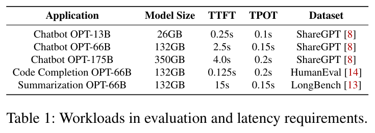
Paper's Table 1. Chatbot (ShareGPT) has balanced TTFT/TPOT; code completion (HumanEval) demands very low TTFT (0.125 s), so both systems become TTFT-bound; summarization (LongBench) has loose TTFT (15 s) but stringent TPOT (0.15 s), isolating decode quality — the regime where colocation hurts most.
End-to-end chatbot gains across model scales:
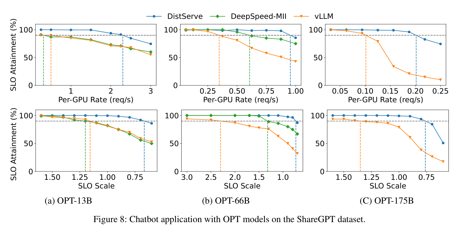
Paper's Figure 8: (a) OPT-13B, (b) OPT-66B, (c) OPT-175B; vertical line = max per-GPU rate meeting 90% attainment. DistServe sustains 2.0–4.6× vLLM's rate. DeepSpeed-MII narrows the gap on larger models because chunked-prefill partially masks interference — but chunked prefill is slower than full prefill, so MII sacrifices TTFT.
The regime where the split matters most — code completion (TTFT-bound) vs summarization (TPOT-bound):
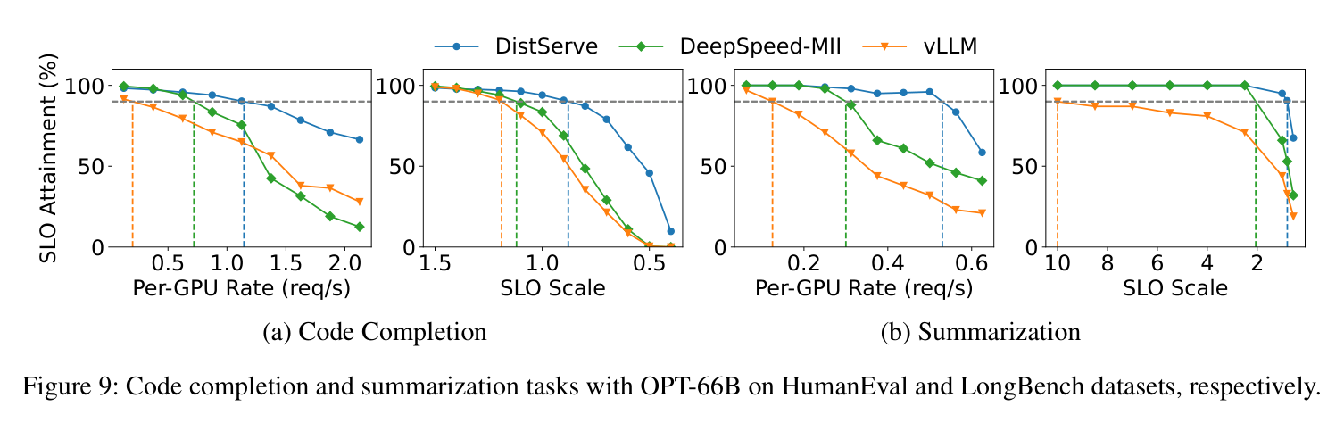
Paper's Figure 9: (a) Code Completion (HumanEval), (b) Summarization (LongBench). Summarization is the extreme: 4.3× rate and 12.6× tighter SLO vs vLLM, because vLLM's colocated decode is dragged by long prefills and fails TPOT, exactly the coupling §2.3 predicts.
Attributing the gain — latency breakdown:
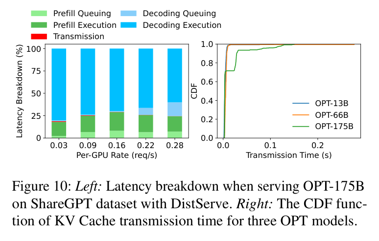
Paper's Figure 10: Left = 5-stage latency breakdown for OPT-175B on ShareGPT; Right = CDF of KV-cache transmission time for three OPT models. KV transfer is <0.1% of total latency and >95% of requests transfer in <30 ms despite the 25 Gbps cross-node testbed — the payoff of segment colocation (§4.2).
Ablation — is it disaggregation or just parallelism tuning?
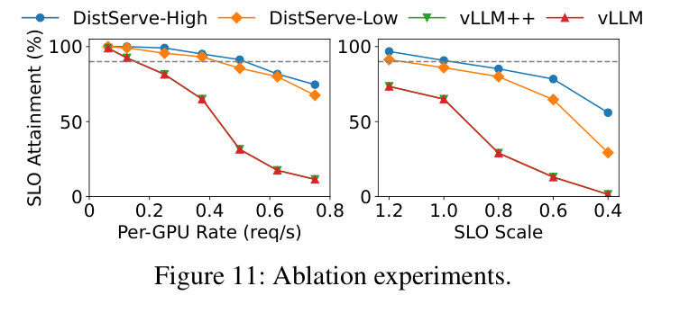
Paper's Figure 11: Ablation experiments. "vLLM++" (best parallelism search under colocation) ≈ plain vLLM, proving parallelism tuning alone yields nothing; DistServe-High (unconstrained placement) > DistServe-Low (segment-colocation constrained), quantifying the price of the NVLINK constraint.
Simulator fidelity (justifies simulation-based ablation):
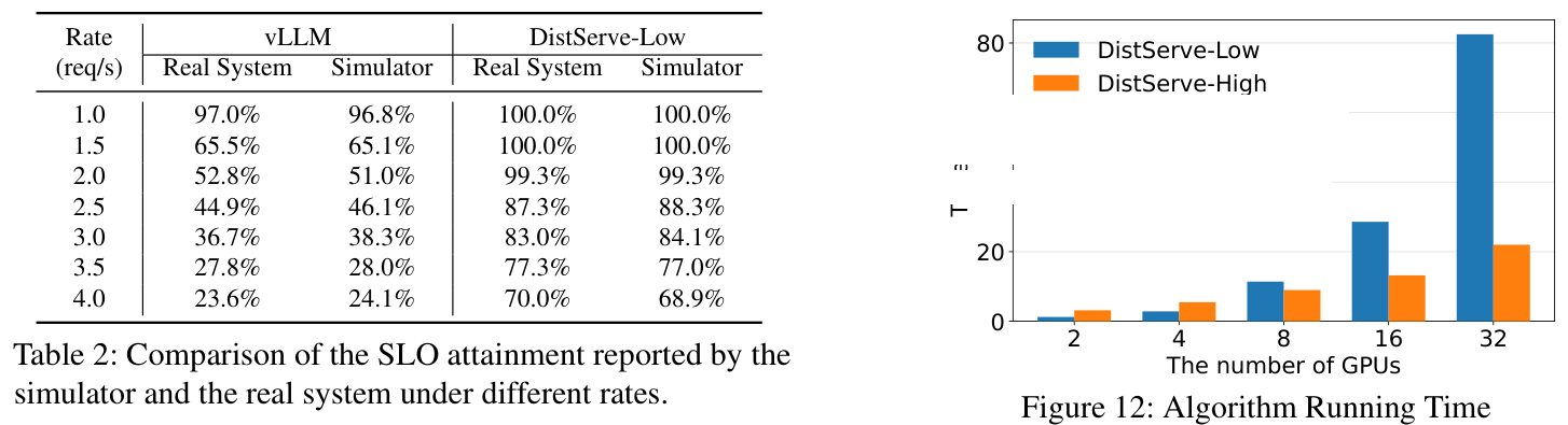
Paper's Table 2. Simulator vs real SLO attainment agrees within <2% across rates for both vLLM and DistServe-Low.
Baseline fairness / metric definitions. Baselines are vLLM [PagedAttention] with intra-op = 1/4/8 for the three OPT sizes (per prior work), and DeepSpeed-MII (chunked-prefill); MII cannot serve OPT-175B due to a
vocab_size/intra_opdivisibility kernel constraint. Metric is SLO attainment (fraction of requests meeting both TTFT and TPOT), and "goodput" is per-GPU requests/s at ≥90% attainment — not raw output tok/s. FP16 throughout; OPT (classic MHA) is chosen deliberately to maximize KV transfer pressure (GQA/MQA models would look even better).6. 论证链 #
Step Claim Support (paper-internal) 1 Prefill is compute-bound, decoding memory-bound — fundamentally different characteristics. §2.1; a 512-token 13B prefill saturates an A100, decode is bandwidth-bound (Fig.3). 2 Colocating them causes interference: prefill stalls decode (TPOT↑), decode inflates prefill (TTFT↑). §2.3, Fig.2 (batch exec-time grows when a prefill job is added). 3 Colocation also couples resource + parallelism plans, forcing over-provisioning to meet the harder SLO. §2.3 para 5; each phase prefers a different parallelism. 4 Therefore disaggregate onto separate instances; each phase optimizes its own SLO independently. §2.3 opportunity + §3.1/§3.2 per-phase analysis. 5 Optimal per-phase parallelism is not fixed: intra-op wins at low rate/tight SLO, inter-op at high rate. Eq.2 vs Eq.3 crossover; Fig.4(a), Fig.5. 6 Since no closed-form SLO attainment exists for real workloads, use a simulator + enumerate placements. §4.1 Algorithm 1, $O(NM^2)$; simulator validated <2% (Table 2). 7 On low-bandwidth clusters, colocate same-stage prefill/decode segments to keep KV transfer on NVLINK. §4.2 Algorithm 2 (instance-segment insight). 8 Net effect: transfer becomes negligible and per-GPU goodput rises up to 7.4×. §6.2 results + §6.3 breakdown (<0.1% transfer). 7. 实现 cross-reference #
Implementation is public:
github.com/LLMServe/DistServe. From the paper (§5): the algorithm module + RESTful frontend + orchestration layer are 6.5K lines of Python; the parallel execution engine is 8.1K lines of C++/CUDA. The frontend is OpenAI-API-compatible (sampling params like max output length, temperature). The orchestration layer handles request dispatch, KV transmission (NCCL cross-node, asyncCudaMemcpyintra-node), and result delivery. Each instance uses Ray actors for GPU workers and integrates continuous batching, FlashAttention, and PagedAttention; supports OPT and LLaMA. Specific file:line citations are[实现未公开]in the paper text itself, but the repository above is the authoritative source.核心技术壁垒 (dedicated paragraph). The hardest-to-replicate piece is Algorithm 2's instance-segment colocation, not the disaggregation idea per se (concurrent works Splitwise/TetriInfer/DéjàVu also disaggregate). The subtlety: naively colocating whole prefill+decoding instances on one node fails for large models — two OPT-175B replicas (350 GB ×2) exceed an 8×80 GB node (640 GB). DistServe instead exploits that KV transfer is stage-local: split each instance into inter-op stage segments and colocate only the matching-stage prefill and decoding segments per node, so transfer is always NVLINK-local regardless of total model size. This constraint is folded into the parallelism search (
get_intra_node_configs, the $P_p.num\_gpus + P_d.num\_gpus \le M$ guard), not applied afterward — reproducing it means jointly searching parallelism and placement under a per-node GPU budget, which is why a black-box disaggregation clone underperforms DistServe-High-style unconstrained placement but the constrained search still recovers most of the benefit.关键实现细节 (easy-to-miss tricks):
- Pull-based KV transfer — decoding instances fetch KV on demand and the prefill instance's HBM doubles as a queuing buffer. This is what prevents burst-induced memory overload on decode instances; a push design would OOM under bursty arrivals.
- Token-count batch balancing via $L_m$ — prefill batches are packed to a total sequence length near the GPU-saturation threshold $L_m$ (batch multiple short requests, or run a long request alone); decode uses $L_m$ as max batch size. Since new-token count reliably predicts batch execution time, this keeps pipeline stages balanced and suppresses bubbles without an explicit scheduler model.