DynaServe: Unified and Elastic Execution for Dynamic Disaggregated LLM Serving #

Chaoyi Ruan, Yinhe Chen, Dongqi Tian, Yandong Shi, Yongji Wu, Jialin Li, Cheng Li | 2025-04 | https://arxiv.org/abs/2504.09285 Category: framework | Tags: serving, scheduling, disaggregation, SLO-aware, KV-cache Read: 2026-04-16

核心三问 #

Q1: 这篇论文试图解决什么核心痛点/问题？

LLM推理必须同时满足严格延迟SLO（如100ms P99 TBT）和高吞吐量（goodput），但现实工作负载中prompt和response长度的动态变化导致prefill（计算密集）和decode（内存密集）两阶段严重失衡。现有的colocation方案（即使使用chunked prefill）会造成prefill-decode干扰导致尾延迟炸裂（P99 TBT>300ms），而disaggregation方案虽然避免了干扰但GPU利用率极低（MFU低至0.2%），两种方案都无法在动态不平衡负载下同时实现低延迟和高吞吐。

Q2: 作者提出了什么新的"杀手锏"方法/架构？

作者提出DynaServe，核心创新是微请求(micro-request)抽象和自适应分区调度(APS)。不同于传统方案只能在prefill/decode边界分割请求，DynaServe可以在任意token边界将请求拆分为两个协作的$\alpha$/$\beta$微请求。通过两级调度框架——全局调度器用二分搜索快速找最优分割点平衡GPU间负载，本地调度器基于运行时profiling动态组合SLO-aware batch——统一了colocation和disaggregation两种范式为同一泛化执行空间的特例。

Q3: 最终效果/结论如何？

在A100集群上使用真实工作负载（BurstGPT、Azure Code等）评估，DynaServe将服务容量提升1.15x-3.07x（对比colocation）和1.09x-1.67x（对比disaggregation），goodput提升最高1.91x和1.61x，混合负载下性能提升60%，同时保持高SLO达标率。

逻辑故事还原 #

背景 (Context) #

LLM推理天然分为两阶段：prefill处理全部输入tokens生成KV cache（计算密集，GPU利用率高），decode逐token生成输出（内存密集，GPU计算单元大量空闲）。现有方案面临两难：

• Colocation（同置）：将prefill和decode放在同一GPU上。优点是简单且GPU利用率均衡，但长prefill会阻塞decode步骤，导致尾延迟飙升。即使引入chunked prefill将长prompt分段，效果也依赖chunk size超参数，且对动态负载无能为力。
• Disaggregation（分离）：将prefill和decode分配到不同GPU池。完全消除了干扰，但只有在两阶段负载完美平衡时才高效——现实中几乎不可能。资源碎片化严重：一台GPU MFU 43%而另一台仅0.2%。

真实trace分析表明：Azure Code是持续prefill偏重的，BurstGPT在prefill偏重和decode偏重之间剧烈波动——没有一种静态方案能hold住。

破局 (Insight) #

作者的关键洞察是：为什么请求只能在prefill和decode的边界处分割？ 如果能在任意token位置分割——比如把一部分decode工作merge到prefill GPU上，或者把部分prefill offload到decode GPU上——就能像调音台一样动态调节每台GPU的工作比例。

👉 生活化类比：想象一家餐厅有两个厨师。传统disaggregation是"厨师A只做前菜，厨师B只做主菜"——如果今天客人都点主菜，厨师A就闲着。DynaServe的做法是：任何厨师可以做任何菜的任何部分，根据实时订单量动态分配任务，甚至一道菜的前半部分由A做、后半部分由B做。

拆解 (Deconstruction) #

1. 微请求抽象：将每个请求的$L=P+D$ tokens在任意分割点$s$处切成$\alpha$（tokens $1 \ldots s$）和$\beta$（tokens $s+1 \ldots L$）两个微请求。$s=P$时退化为disaggregation，$s=L$时退化为colocation——两种传统方案都是micro-request的特例。
1. 全局调度器：对每个到达的请求，以PD disaggregation比例$\phi=P/(P+D)$为起点，用有界二分搜索（最多$K=6$步）找到让两台GPU执行时间差最小化的最优$\phi$。每步probe仅需几微秒（离线profiling + LRU cache查表），考虑了所有GPU的实时负载。
1. 本地调度器：每个GPU实例上独立运行SLO-aware batch组合。先加入所有decode请求（延迟敏感），然后查询profile table确定在当前decode负载下允许混入的最大prefill token预算$M$，贪心填充prefill请求直到预算耗尽。Profile table由实际运行时延不断更新校准。
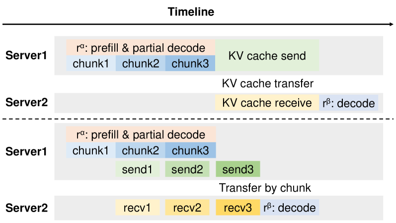
1. Chunk-based KV Transfer：$\alpha$微请求处理完一个chunk后，其KV block立即DMA推送到$\beta$所在GPU，与下一个chunk的计算重叠，非重叠传输减少94%。

核心图表 #

Figure 1: Throughput vs. SLO Attainment Trade-off #



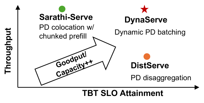
What it shows: 三种服务架构（PD Colocation、PD Disaggregation、DynaServe）在吞吐量和SLO达标率两个维度上的trade-off。

Why it matters: 这是论文的motivation图，清晰展示了colocation追求高吞吐但牺牲SLO（左上方），disaggregation满足SLO但吞吐低（右下方），DynaServe向右上方推进pareto frontier。

Detailed description: X轴为SLO attainment（SLO达标率），Y轴为throughput。PD Colocation with chunked prefill达到较高吞吐但SLO达标率极低；PD Disaggregation保持高SLO达标率但吞吐量受限；DynaServe在两个维度上同时表现优异，占据右上角的pareto最优区域。图中绿色箭头标注了DynaServe相对于两个baseline的改进方向。

Figure 4: DynaServe Architecture #



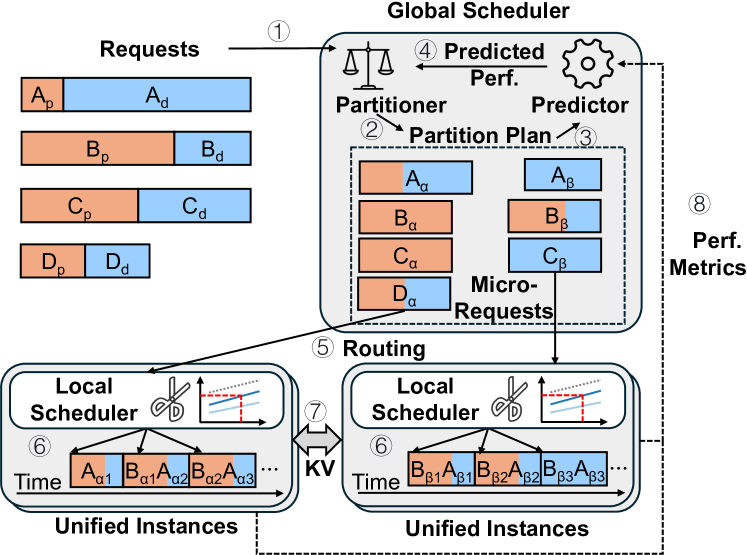
What it shows: DynaServe的完整系统架构，包括微请求分割、两级调度、统一GPU实例、KV cache传输。

Why it matters: 这是论文的"灵魂图"，展示了整个系统的数据流和控制流。

Detailed description: 图中左侧是Request Queue，请求到达后经过全局调度器①。全局调度器执行三个关键步骤：②计算分割比例$\phi$，③预测两台GPU的执行时间$T_1$和$T_2$，④选择最优分割。分割后的$\alpha$和$\beta$微请求被路由⑤到统一的GPU实例。每个GPU实例有本地调度器⑥负责SLO-aware batch组合。当微请求跨实例时，通过RDMA进行KV cache传输⑦。全局调度器还通过⑧收集各GPU的运行时统计。橙色表示prefill阶段，蓝色表示decode阶段。四个示例请求(A-D)展示了不同的分割模式：A和B跨GPU分割（混合prefill+decode），C是标准PD disaggregation，D完全在一个GPU上执行（colocation）。

Figure 6: Batch Composition Impact on Latency and Utilization #



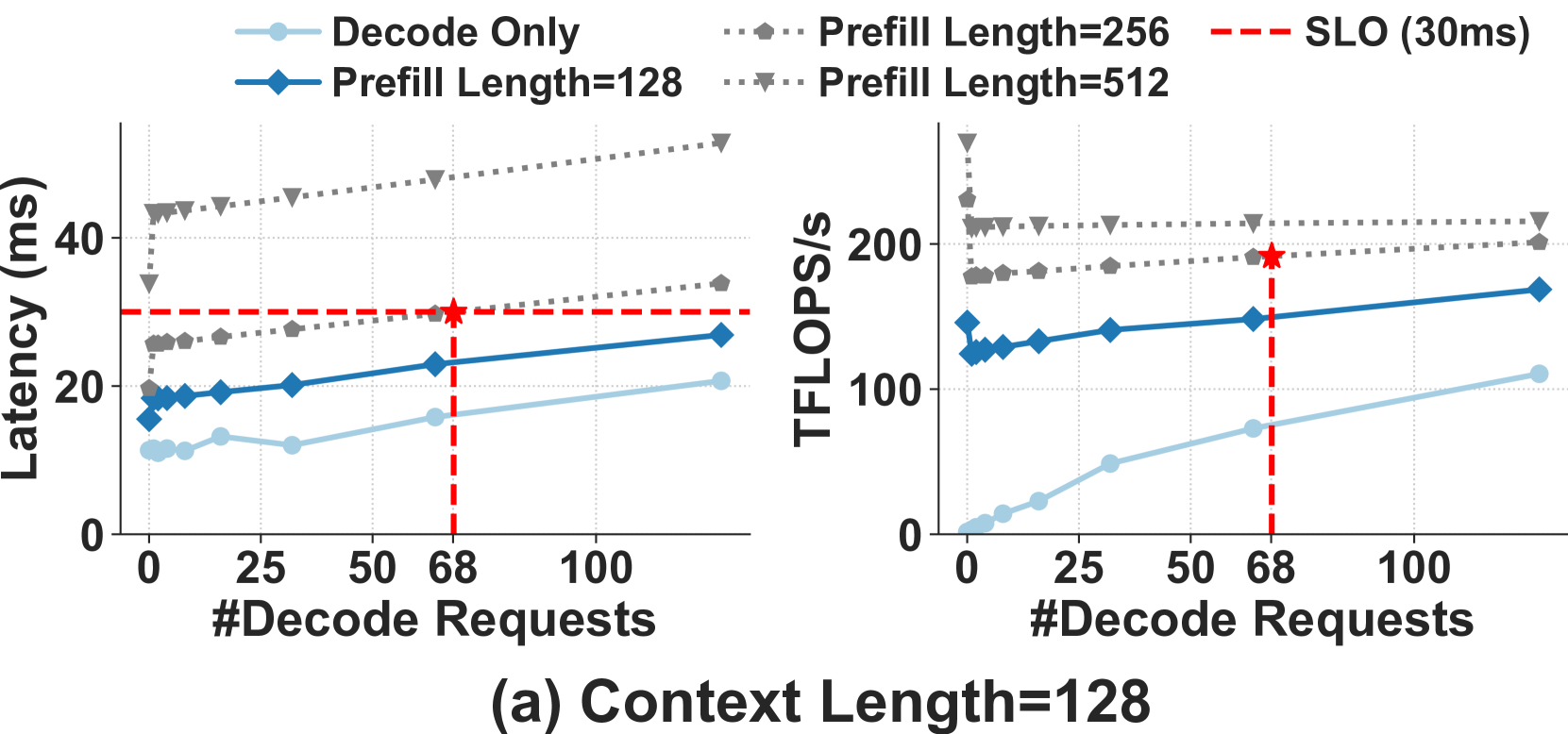
What it shows: 在不同batch组合策略下，Llama-3.1-8B在A100上的延迟（左）和GPU计算利用率（右），分别在短context（128 tokens，上排）和长context（1024 tokens，下排）场景下的表现。

Why it matters: 这张图揭示了prefill-decode混合batch中的核心trade-off，是local scheduler设计的理论基础。

Detailed description: 每张图中，X轴是并发decode请求数，Y轴分别是延迟(ms)和TFLOP/s。红色虚线标记SLO阈值。不同曲线代表不同prefill chunk大小（0/256/512/1024 tokens）。关键观察：(1) decode-only batch满足SLO但GPU利用率低；(2) 混入prefill提升利用率但增加延迟；(3) Latency-Constrained Utilization (LCU) point标记了SLO约束下的最优运行点；(4) 最优batch组合随context长度和decode数量动态变化。

Figure 8: Goodput Comparison (Main Results) #



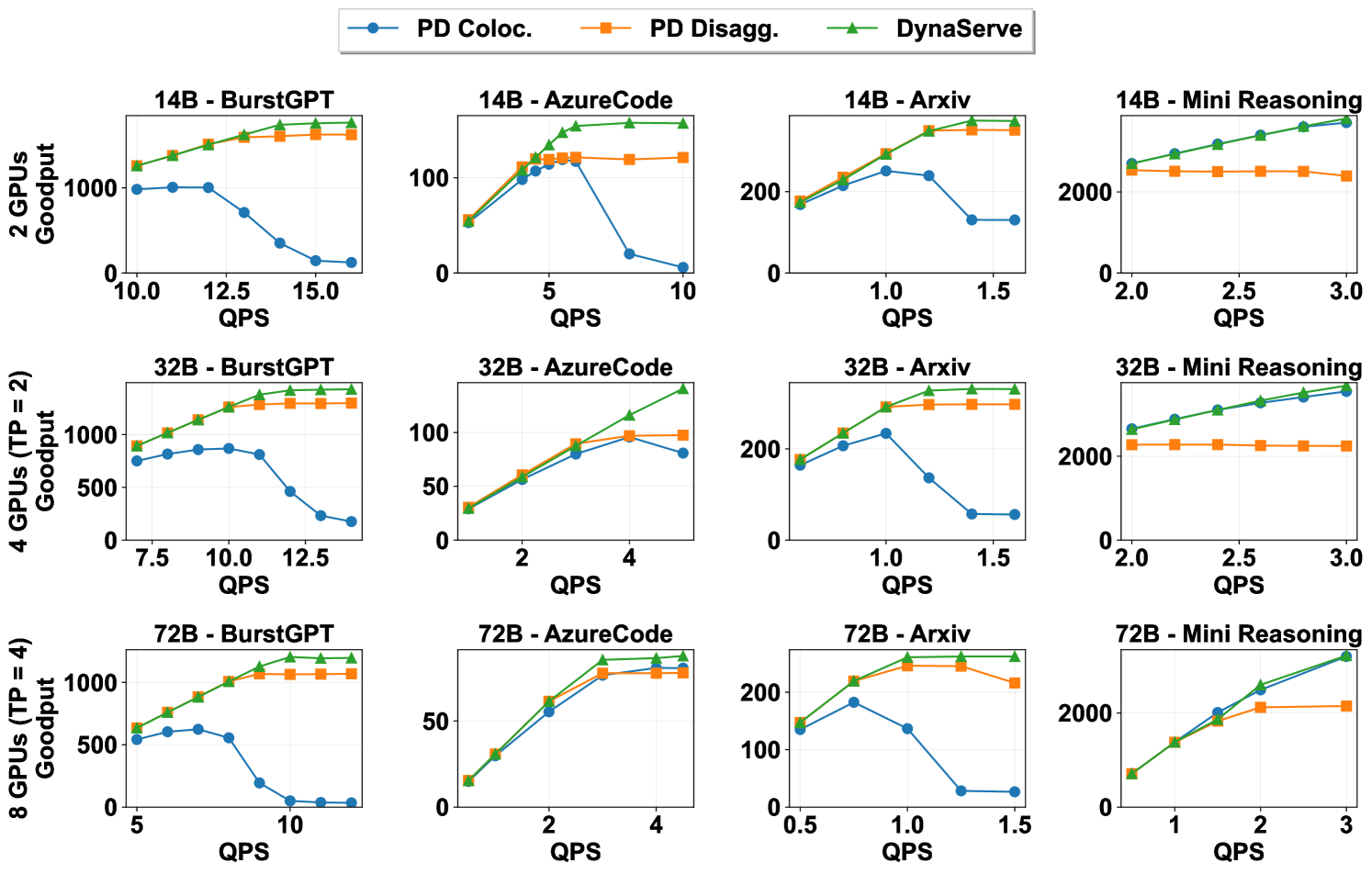
What it shows: DynaServe、PD Colocation、PD Disaggregation在四种真实工作负载（BurstGPT、Azure Code、arXiv Summarization、Mini Reasoning）和三种模型规模（14B、32B、72B）下的goodput对比。

Why it matters: 这是论文的主实验结果图，全面展示了DynaServe在多种场景下的性能优势。

Detailed description: 3行（模型大小）×4列（工作负载）的子图矩阵。每个子图X轴为QPS（请求到达率），Y轴为goodput（token/s under SLO）。三条曲线分别对应三种系统。DynaServe（绿色/蓝色）在所有12个配置中一致性地达到最高goodput，最大改进91%（vs colocation）和61%（vs disaggregation）。Colocation在高QPS时因PD干扰导致goodput急剧下降，disaggregation因GPU利用率不均而提前饱和。

Figure 9: Serving Capacity #



What it shows: 三种系统在四种工作负载下使用Qwen-14B时的最大可持续QPS（在P99 TBT < 100ms SLO约束下）。

Why it matters: Serving capacity是比goodput更严格的SLO-constrained指标（只允许1%违规），展示了系统在严格延迟约束下的真实服务能力。

Detailed description: 四组柱状图，每组三根柱子。DynaServe平均支持2.37x于colocation和1.37x于disaggregation的QPS。在Azure Code（prefill偏重）负载下优势最明显，达到约3x。在Mini Reasoning（decode偏重）下colocation表现相对好但DynaServe仍领先。

Key Tables #

Table 1: GPU Resource Utilization Comparison #

Metric	P-8192, D-32		P-2048, D-512		P-219, D-1467
	Disagg.	Coloc.	Disagg.	Coloc.	Disagg.	Coloc.
MFU (%) G1	43.24	38.94	30.59	21.26	2.09	13.98
MFU (%) G2	0.19	38.94	7.93	21.26	14.34	13.98
p99-TBT (ms)	58.09	352.93	65.11	336.81	74.47	162.67
Attainment (%)	100.00	1.73	99.83	84.09	99.95	94.46

Takeaway: Disaggregation满足SLO但GPU利用极度不均（G1 MFU 43% vs G2 0.2%），Colocation利用均衡但SLO达标率极低（最差仅1.73%）——这个"两难困境"就是DynaServe要破解的。

Table 2: Hybrid Workload Performance #

System	PD Coloc.	PD Disagg.	DynaServe
Serving Capacity (rps)	4.6	5.9	7.4
Goodput (token/s)	316.32	399.31	473.84

Takeaway: 在混合工作负载（50% BurstGPT + 50% Azure Code）下，DynaServe的serving capacity比colocation高60%，比disaggregation高25%，展示了对异构流量的强适应能力。

Table 3: Scheduling Overhead #

QPS	6	8	10	12	14	16
Overhead (ms)	17.47	15.48	14.40	13.70	14.85	14.54

Takeaway: 每个请求的全局调度开销始终<20ms，而请求的端到端延迟约5000ms（10 QPS时），调度开销可忽略不计。

关键细节与启示 #

技术细节补充:

1. 全局调度器的二分搜索以PD disaggregation比例$\phi=P/(P+D)$为起点，每步probe仅需μs级（基于离线profiling的LRU cache查表），且考虑当前所有GPU实例的实时排队和负载情况，不只是孤立优化单个请求。
2. 本地调度器的profile table记录(plen, ctx, dnum, time)四元组，在运行时不断用实际batch延迟更新校准，实现了"自校准"的延迟预测——这比静态的chunk size配置灵活得多。

一句话总结: DynaServe通过micro-request抽象在任意token边界动态分割请求，配合两级（全局负载均衡+本地SLO-aware batching）调度框架，将colocation和disaggregation统一为泛化执行空间的特例，在动态不平衡负载下同时实现了低尾延迟和高吞吐。

Core Contribution #

A micro-request abstraction that splits LLM requests at arbitrary token boundaries with a two-level scheduling framework, unifying colocation and disaggregation paradigms for maximizing goodput under strict SLO constraints.

Summary #

LLM serving faces a fundamental tension between low tail latency (required for SLOs like 100ms P99 TBT) and high throughput (for cost efficiency). Colocation approaches suffer from prefill-decode interference causing SLO violations (P99 TBT >300ms), while disaggregation wastes GPU resources due to workload imbalance (MFU as low as 0.2%). Real-world traces show persistent and time-varying skew between prefill and decode demands.

DynaServe introduces the micro-request abstraction, allowing any request to be split at any token boundary into two cooperating segments ($\alpha$ and $\beta$). A global scheduler uses binary search with a lightweight execution predictor to find optimal split points that balance load across unified GPU instances. Local schedulers on each GPU independently compose SLO-aware batches by dynamically adjusting prefill-to-decode token ratios based on runtime profiling. Chunk-based KV cache transfers overlap communication with computation, reducing non-overlapped transfer by 94%.

Evaluated on A100 clusters with real-world traces (BurstGPT, Azure Code, arXiv Summarization, Mini Reasoning), DynaServe achieves 1.15x-3.07x higher serving capacity and up to 1.91x/1.61x higher goodput compared to colocation/disaggregation baselines. In hybrid workloads, it improves performance by 60%.

Key Findings #

• Neither colocation nor disaggregation handles dynamic unbalanced workloads well — colocation violates SLOs (P99 TBT >300ms), disaggregation wastes GPU resources (MFU as low as 0.2%)
• Micro-request abstraction generalizes both paradigms — colocation and disaggregation are special cases of the broader partitioning space
• Two-level scheduling achieves near-optimal performance with <20ms per-request overhead (6-step binary search with μs-level probes)
• SLO-aware local batching raises SLO attainment from 52% to 99% by dynamically controlling prefill budget per batch
• Chunk-based KV transfer reduces non-overlapped transfer time by 94%
• DynaServe is robust to output length prediction errors (only 2.9% goodput drop at $\sigma=100$ tokens)

Limitations #

• Requires output length prediction which introduces error (though shown to be tolerant)
• Evaluated only on A100 GPUs — unclear performance on other hardware (H100, MI300X)
• Built atop vLLM — porting to other engines may require significant effort
• Limited to two-way splits ($\alpha$/$\beta$) — multi-way partitioning unexplored
• Cross-instance KV transfers still add overhead especially for large models
• No evaluation with speculative decoding or other advanced inference techniques
• Open-source code not yet released at time of publication

Infrastructure Impact #

• Algorithm: N/A — no new training algorithms; purely an inference-time system optimization
• Kernel: Does not require custom GPU kernels; uses existing vLLM/PyTorch kernels and NCCL for transfers. Chunk-based KV transfer could benefit from custom RDMA kernels for further optimization.
• Framework: Core contribution — introduces micro-request abstraction and two-level scheduling that unifies colocation and disaggregation for LLM serving. Directly applicable to any vLLM-based deployment.
• LLM: Model-agnostic serving approach tested on Qwen-2.5 series (14B/32B/72B); works with any autoregressive LLM that has standard prefill+decode phases.
• Agent: Supports strict latency SLOs (100ms P99 TBT) enabling responsive agent-serving; dynamic workload adaptation is valuable for bursty, heterogeneous agent traffic patterns.
• Cluster: Leverages multi-GPU clusters with RDMA for KV cache transfer; unified GPU pool abstraction eliminates need for static prefill/decode GPU allocation.

---

Deep Analysis (framework) #

1. System Scope #

• Primary goal: Online LLM inference serving — maximizing goodput (tokens/s under SLO) while maintaining strict latency SLOs (100ms P99 TBT)
• Distributed: Multi-GPU, multi-node. Tested on 2 servers × 4 A100 GPUs, scaled up to 8 GPUs with TP=4
• Online, latency-sensitive: Targets interactive real-time serving with P99 TBT < 100ms
• Workload: Standard autoregressive LLM inference (prefill + decode) with dynamic, unbalanced request patterns

2. Architecture & Data Flow #

2a. End-to-End Data Flow #

Figure 4: DynaServe Architecture #



解读: 这张架构图展示了完整的请求生命周期。请求从左侧Queue进入全局调度器，经历分割决策后被路由到两个统一GPU实例。$\alpha$微请求先执行，产生的KV cache通过RDMA chunk-by-chunk传输到$\beta$实例。本地调度器在每个实例上独立组合batch。关键设计：所有GPU实例是对等的——任何实例可以处理任何类型的微请求，这是DynaServe区别于disaggregation（固定角色分配）的根本。

[Request Arrival] → [Global Scheduler: binary search for ϕ] → [Split into rα + rβ]
                      ↓ O(1) per request, <20ms
[rα → GPU Instance A] → [Local Scheduler: SLO-aware batch] → [Execute prefill+partial decode]
                            ↓ profile table lookup
[KV Cache: chunk-based DMA push] ─── RDMA ───→ [GPU Instance B]
                                                  ↓
[rβ → GPU Instance B] → [Local Scheduler: SLO-aware batch] → [Execute remaining decode]
                                                                ↓
                                                          [Return tokens to client]

Stage	Input → Output	Location	Latency	Data format
Global scheduling	Request $(P,D)$ → ($r_\alpha$, $r_\beta$, routing)	CPU	<20ms	Split point $s$, GPU assignment
Prefill ($r_\alpha$)	Prompt tokens → KV cache + first tokens	GPU HBM	varies by P	[layers, heads, seq, dim]
KV Transfer	KV blocks → remote GPU	NIC/RDMA	overlapped	Chunk-sized KV blocks
Decode ($r_\beta$)	KV cache + context → output tokens	GPU HBM	~30-50ms/step	[vocab_size] per token
Local batch formation	Pending requests → batch	CPU (per-GPU)	~μs	(plen, ctx, dnum) tuple

Control plane: Global scheduler (centralized, CPU-side) + runtime statistics collection (⑧ in Figure 4)

Data plane: GPU instances execute micro-requests, RDMA transfers KV cache

Stateful: KV cache on each GPU instance; global scheduler maintains per-GPU load estimates

Stateless: Request routing decisions are made per-request, no cross-request state

Failure handling: Not explicitly discussed in the paper — a notable gap for production deployment.

2b. Data Movement Hotspots #

1. KV Cache Transfer (GPU↔GPU via RDMA): When $r_\alpha$ and $r_\beta$ are on different GPUs, the full KV cache for the $\alpha$ segment must be transferred. For a request with P=1024 prefill tokens on Qwen-2.5-14B, this is ~hundreds of MB per request. Happens once per request split. DynaServe overlaps this with chunk-based transfer (94% reduction in non-overlapped time).
1. HBM Bandwidth for Decode: Each decode step reloads the entire growing KV cache from HBM. For long sequences (>1000 tokens), this dominates decode latency. Happens once per output token. Not overlapped — this is the fundamental memory-bound bottleneck of decode.
1. Model Weight Loading: All GPU instances load full model weights. For TP configurations, weights are sharded across GPUs within a TP group. Happens once at startup. Not a runtime bottleneck.

3. Key Innovations #

Innovation	Mechanism	Benefit	Cost/Tradeoff
Micro-request abstraction	Split request at arbitrary token boundary into $\alpha$/$\beta$ segments	Generalizes colocation & disaggregation; enables fine-grained load balancing	Added complexity in scheduling; requires output length prediction
Global binary search scheduler	Bounded binary search ($K=6$ steps) over split ratio $\phi$ with execution predictor	Near-optimal split in $O(1)$ time, <20ms overhead	Relies on accuracy of execution predictor; prediction errors possible
SLO-aware local batching	Profile table tracks (plen, ctx, dnum, time); dynamically caps prefill budget $M$	Raises SLO attainment from 52% → 99%; adapts to runtime conditions	Profile table needs warm-up period; may be conservative early on
Chunk-based KV transfer	DMA-push completed KV chunks while computing next chunk	94% reduction in non-overlapped transfer; overlaps comm with compute	Requires RDMA infrastructure; adds coordination complexity

4. Scheduling & Resource Management #

• Batch formation: Dynamic, continuous batching with SLO-aware composition. Not static chunk sizes — the prefill budget $M$ is dynamically computed per batch based on current decode load and profile table.
• Memory management: Uses vLLM's PagedAttention for KV cache management. No novel memory management beyond chunk-based transfer.
• GPU utilization: Two mechanisms prevent idle time: (1) Global scheduler balances execution time across GPUs by tuning $\phi$; (2) Local scheduler fills compute gaps by mixing prefill tokens into decode-heavy batches up to SLO limit.

Figure 6: Batch Composition Analysis #



解读: 这张图是local scheduler设计的实验基础。四个子图清晰展示了prefill混入量对延迟和GPU利用率的影响。关键发现：(1) decode-only batch安全但低效（TFLOP/s低）；(2) 混入512 token prefill在短context场景下可在SLO内大幅提升利用率；(3) LCU Point标记了每种配置的最优运行点——local scheduler的目标就是动态逼近这个点。

• Multi-tenancy: Not discussed — single model deployment assumed.
• Priority/SLO-aware: Core feature. Local scheduler uses FCFS by default but is policy-agnostic (can plug in priority, shortest-job-first, or deadline-aware).

5. Target Scenarios & Workload Characterization #

Scenario	Workload Pattern	SLO / Goal	Why existing systems fail
Code completion (Azure Code)	Long prompts, short outputs; prefill-heavy	P99 TBT < 100ms + max goodput	Colocation: PD interference (P99>350ms); Disaggregation: prefill GPU overloaded, decode GPU idle
Chatbot (BurstGPT)	Balanced but bursty; rapid prefill↔decode fluctuation	P99 TBT < 100ms + max goodput	Colocation: tail latency spikes under bursts; Disaggregation: can't adapt to shifting balance
Document summarization (arXiv)	Very long inputs, moderate outputs	P99 TBT < 100ms + max goodput	Both struggle: massive prefill causes interference or overload
Reasoning tasks (Mini Reasoning)	Short prompts, very long outputs; decode-heavy	P99 TBT < 100ms + max goodput	Disaggregation: decode GPU memory saturated; Colocation performs better but still limited
Hybrid production traffic	Mixed workload types	P99 TBT < 100ms + max goodput	Static partitioning cannot serve diverse patterns efficiently

Primary bottlenecks:

• Azure Code / arXiv: Compute-bound (prefill dominates) → disaggregation leaves decode GPU idle
• Mini Reasoning: Memory-bound (long decode sequences) → disaggregation overloads decode GPU
• BurstGPT / Hybrid: Scheduling-bound → static partitioning can't adapt to dynamic shifts

6. Performance Evaluation & Before-After Comparison #

6a. Metrics Definition #

Metric	Definition	Unit	Direction
Goodput	Output tokens generated per second while meeting SLO	tokens/s	Higher ↑
Serving Capacity	Maximum sustainable QPS with P99 TBT < 100ms	rps	Higher ↑
P99 TBT	99th percentile time-between-tokens	ms	Lower ↓
P50 TBT	Median time-between-tokens	ms	Lower ↓
SLO Attainment	Percentage of tokens generated within 100ms TBT	%	Higher ↑
MFU	Model FLOPs Utilization	%	Higher ↑

6b. Before-After Comparison Table #

Figure 8: Goodput Main Results #



解读: 这是论文的核心实验结果。3×4矩阵覆盖了所有模型规模和工作负载组合。DynaServe在所有12个配置中一致性地达到最高goodput。关键观察：(1) Colocation在高QPS时急剧下降（PD干扰），而DynaServe保持平稳plateau；(2) Disaggregation提前饱和因GPU利用不均；(3) 随着模型从14B增大到72B，DynaServe的优势更加明显。

Optimization	Metric	PD Coloc.	PD Disagg.	DynaServe	Improvement	Conditions
Micro-request + APS	Max goodput	baseline	baseline	best	up to 1.91x vs Coloc, 1.61x vs Disagg	Qwen-14B/32B/72B, 4 real workloads, A100
Micro-request + APS	Serving capacity	4.6 rps	5.9 rps	7.4 rps	1.6x vs Coloc, 1.25x vs Disagg	Qwen-14B, hybrid workload
SLO-aware batching	SLO attainment	52% (w/o)	—	99% (w/)	47pp improvement	Qwen-14B, AzureCode, at DynaServe capacity
Chunk-based KV transfer	Non-overlapped transfer	baseline	—	-94%	94% reduction	Mini Reasoning task

Figure 9: Serving Capacity #



解读: 四组柱状图展示了在更严格的serving capacity指标下的对比。DynaServe在所有负载下都领先，平均2.37x于colocation、1.37x于disaggregation。AzureCode负载下优势最大（~3x vs colocation），因为该负载prefill偏重导致colocation干扰最严重。

6c. Bottleneck Shift Analysis #

Before DynaServe:
  Colocation: Memory-bound (PD interference) → P99 TBT > 300ms
  Disaggregation: Scheduling-bound (fixed partition) → GPU underutilization

After micro-request + global scheduling:
  Bottleneck shifts to: Local batch composition (how to mix prefill+decode per batch)

After SLO-aware local batching:
  Bottleneck shifts to: KV cache transfer overhead (cross-GPU communication)

After chunk-based KV transfer:
  REMAINING bottleneck: Output length prediction accuracy + fundamental memory-bandwidth
  limit of decode phase

6d. Baselines & Fairness #

• Fair comparison: Yes — all systems use vLLM as the base engine, same hardware (A100 80GB), same models (Qwen-2.5 series), same workloads.
• Baseline tuning: Colocation chunk sizes tuned between 256-2048 per workload; disaggregation uses advanced v1 scheduling. Fair effort given to baselines.
• Scale: Advantages appear even at 2 GPUs, amplify at 8 GPUs (72B model).
• Framework overhead: Global scheduling <20ms/request (amortized over ~5000ms request lifetime).
• Scenarios where baselines win: Colocation is competitive on Mini Reasoning (decode-heavy, short prefill → less PD interference). Disaggregation is competitive on Azure Code at low QPS (isolation benefit outweighs underutilization at low load).

7. API & Usability #

• API: Built on vLLM — inherits OpenAI-compatible API
• Model format: HuggingFace models via vLLM (Qwen-2.5 series tested)
• Deployment: Multi-server setup with RDMA networking required; 3K lines of Python + C++ global scheduler
• Configuration: Key knobs: K (binary search steps, default 6), $\varepsilon$ (convergence tolerance), prediction margin (20 tokens), profile table warm-up. Relatively low tuning burden compared to manual chunk size tuning.

8. Infrastructure Impact #

Layer	Impact
Algorithm	Does not enable new training paradigms; purely inference-time
Kernel	Uses existing kernels; chunk-based transfer could benefit from custom RDMA kernels
LLM	Supports any autoregressive LLM with standard prefill+decode; tested on Qwen-2.5 14B/32B/72B
Agent	Strict SLO guarantees (100ms P99 TBT) enable responsive agent serving; dynamic adaptation helps with bursty agent traffic
Ops	Requires RDMA networking; runtime statistics collection for scheduler; no explicit monitoring/autoscaling discussion

9. Comparison Matrix #

Feature	DynaServe	vLLM (Coloc.)	vLLM (Disagg.)	DistServe	Splitwise
Continuous batching	✅	✅	✅	✅	✅
Paged attention	✅ (via vLLM)	✅	✅	✅	?
Chunked prefill	✅ (dynamic)	✅ (static)	N/A	N/A	N/A
PD disaggregation	✅ (as special case)	❌	✅	✅	✅
Arbitrary split point	✅	❌	❌	❌	❌
SLO-aware batching	✅ (dynamic profile)	❌ (static chunk)	❌	✅ (static)	❌
Dynamic load balancing	✅ (global scheduler)	❌ (round-robin)	❌ (fixed P/D pools)	❌	❌
KV cache overlap	✅ (chunk-based)	N/A	Layer/iter-level	Layer-level	Layer-level
Multi-node	✅	✅	✅	✅	✅
Speculative decoding	❌ (not evaluated)	✅	?	?	?

10. Adoption & Maturity #

• Open source: Planned but not yet released at time of publication
• Community: New system from NUS + USTC research groups; no established community yet
• Production: No production deployment mentioned; evaluated on research testbed
• Adoption path: Built atop vLLM with 3K lines of code — relatively low integration barrier for vLLM users. Requires RDMA-capable networking between GPU nodes. The non-intrusive design and backend integration interface suggest it could be extended to other engines.