Parallax: Efficient LLM Inference Service over Decentralized Environment
Parallax: Efficient LLM Inference Service over Decentralized Environment — L2 #
§1 TL;DR #
Two-phase DP scheduler converts heterogeneous volunteer GPUs into a practical LLM inference platform: Phase 1 allocates model layers region-locally via DP + water-filling; Phase 2 selects per-request pipeline chains via DAG shortest-path over live DHT metrics. Up to 3.6× throughput over HexGen on 7-GPU decentralized testbed.
§2 痛点 · 方法 · 结果 #
Q1 痛点 #
Centralized LLM serving requires homogeneous GPU clusters with high-bandwidth interconnects — prohibitively expensive for many organizations. Decentralized volunteer GPU pools offer an alternative, but introduce three compounding challenges:
- GPU heterogeneity: volunteer nodes span different compute power (FLOPs), memory capacity, and architecture generations — naive even-layer partitioning creates stragglers.
- Network heterogeneity: inter-node links range from local high-bandwidth to cross-region congested paths (down to hundreds of MB/s); standard collective operations degrade severely.
- Dynamic membership: GPUs join and leave unpredictably, requiring allocation adaptation without full-system disruption.
- DP over sorted GPU capacities explores replication counts $k \in \{1, \dots, k_{\max}\}$
- State $\mathrm{dp_1}(i, \mathbf{r}, f)$: GPU index $i$, residual-layer multiset $\mathbf{r}$, fully-assigned pipeline count $f$
- Three transitions: skip GPU, extend existing pipeline, start new pipeline
- Scoring: $Z(k) = k - \frac{s^{\star}(k)/k \cdot r_{\mathrm{RTT}}}{T_{\mathrm{comp}}}$ trades off replications (throughput) against communication overhead
- Water-filling rebalances layer assignments within each pipeline to equalize stage execution times
- Heuristics: region-bounded allocation (no cross-region stages) + latency-dominant (minimize stage count)
- Builds layer-indexed DAG from Phase 1 placement; nodes = $(\ell, g_i)$, edges = valid layer transitions
- DHT stores live profiling: $\tau_{g_i}$ (per-GPU processing latency) and $\rho_{g_i, g_{i'}}$ (inter-GPU RTT), updated every 1–2 s
- Single-pass DP sweep: $\mathrm{dp_2}(\ell{+}1, g_{i'}) = \min(\mathrm{dp_2}(\ell{+}1, g_{i'}),\; \mathrm{dp_2}(\ell, g_i) + \rho_{g_i, g_{i'}} + \tau_{g_{i'}})$
- Backtrack extracts minimum-latency chain; chain pinned for session duration
- Complexity: $\mathcal{O}(L\bar{R}^2)$ time, $\mathcal{O}(L\bar{R})$ space
- Throughput: up to 3.6× (avg 1.58×) higher than HexGen — largest gains on 32B model with WildGPT at high request rates (264% improvement)
- Latency: up to 3.2× (avg 1.66×) lower — most pronounced at tail (p99) under communication-dominated regimes
- Scheduling overhead: Phase 1 completes in 8.55 ms at 256 GPUs; Phase 2 adds 6.63 ms/req at 256 GPUs — negligible vs. inference latency
- Testbed: 5× RTX 5090 + 2× RTX 4090, geographically distributed, 10 ms average inter-machine latency
- 符号一致性: all 14 symbols used consistently across Phase 1 (§3.2) and Phase 2 (§3.3); $k$, $L$, $c_i$ carry identical meaning in both phases. ✓
- 边界行为: when $r_{\mathrm{RTT}} = 0$ (zero communication cost), $Z(k) = k$ — pure throughput scaling, optimal at $k = k_{\max}$. When $r_{\mathrm{RTT}} \gg T_{\mathrm{comp}}$, the penalty term dominates and $Z(k)$ collapses, favoring $k = 1$ with minimal stages. This matches the latency-dominant heuristic design. ✓
- 单调性 / 最优结构: $Z(k)$ is not monotonically increasing in $k$ because $s^{\star}(k)/k$ can increase as more replicas require more stages per replica (capacity fragmentation). An interior optimum $\hat{k}$ balances throughput gain against communication cost — the system does not always maximize $k$. ✓
- 量纲分析: $s^{\star}(k)/k$ is dimensionless (stages/replica), $r_{\mathrm{RTT}}/T_{\mathrm{comp}}$ is dimensionless (time/time). Their product is dimensionless, subtracted from $k$ (count). $Z(k)$ has units of "effective replications." ✓
- DP 正确性: Phase 2 recurrence is a Bellman equation on a DAG with non-negative edge weights. Single forward pass (layer 1 → $L$) suffices because the DAG is topologically ordered by layer index — no cycles possible. Backtracking through parent pointers yields the unique optimal path. ✓
- 阶估计验证: with 7 GPUs and $\bar{R} \approx 2$–3 replicas per layer, Phase 2 runs in $\mathcal{O}(L \cdot 9) \approx 576$ operations for Qwen3-32B (64 layers). At 0.01 ms reported (Fig 5, 4 GPUs), this is consistent with sub-microsecond per DP step. At 256 GPUs with $\bar{R} \approx 8$, growth to 6.63 ms/req matches $\mathcal{O}(L\bar{R}^2)$ scaling. ✓
- NP-hardness of joint optimization (§3.1): claimed without formal reduction or proof.
- Water-filling binary search on $\lambda$: no convergence analysis or iteration bound provided.
- DHT staleness impact: 1–2 s profiling interval vs. sub-second inference latencies — no sensitivity analysis.
- 硬件: 5× RTX 5090 + 2× RTX 4090, geographically separated, average 10 ms inter-machine public-network latency
- 模型: Qwen3-32B at BF16 (32B params) and FP8 (16B params)
- 负载: subsampled ShareGPT and WildGPT traces (real ChatGPT conversations)
- 基线: HexGen — heterogeneous LLM inference with static tensor + pipeline parallelism partitioning
- 指标: throughput (req/s), percentile latencies (avg, p95, p96, p97, p98, p99, p100)
- Phase 1 granularity: per-configuration (rerun on membership change)
- Phase 2 granularity: per-request; chain pinned for entire session duration
- No preemption: once a chain is selected, the request runs to completion on that chain
- No admission control or backpressure under overload described
- No per-client or per-priority fairness guarantees
- Step 2 → 3: NP-hardness is claimed without proof; the heuristics' optimality gap relative to an exact solution is unknown.
- Step 5: DHT profiling every 1–2 s may be too coarse for sub-10 ms inference decisions; staleness effects not analyzed.
- Step 6: testbed has only 7 GPUs; Fig 5 shows scheduling scales to 256 GPUs, but end-to-end performance at that scale is unverified.
- Missing comparison: Helix (heterogeneous GPU serving via max-flow, ASPLOS 2025) is a direct competitor omitted from experiments.
- Region-based allocation constraint: Phase 1 forces all stages of each pipeline within the same geographic region as a hard constraint in the DP state transitions — the search space never explores cross-region stage assignments. This single heuristic eliminates the most expensive communication edges (cross-region links at hundreds of MB/s) from the problem, producing the compact DAG that Phase 2 depends on.
- DHT temporal feedback loop: when a GPU chain is selected or released, the GPUs on that chain immediately publish updated $\tau$ values. This creates a fine-grained load-balancing signal beyond the coarse 1–2 s profiling interval — newly loaded GPUs report higher $\tau$, causing Phase 2 to route subsequent requests away. The dual-timescale design (coarse profiling + event-driven updates) is the mechanism behind implicit load balancing without an explicit load balancer.
- 服务阶段: prefill + decode (standard autoregressive generation)
- 并发模式: request-level DP across replicas; no intra-request tensor parallelism
- 硬件亲和性: benefits GPUs with high compute-to-memory ratio; largest gains when inter-node bandwidth is the bottleneck (WAN / decentralized)
- 生态集成: standalone system with custom scheduler and runtime; not a plugin for vLLM / SGLang / TRT-LLM; adoption requires the full Parallax stack
- 局限: no continuous batching described; chain pinned per session (no mid-generation rerouting); no KV cache management innovation beyond standard per-GPU allocation
Prior work (Petals) demonstrated feasibility of volunteer-driven LLM inference but used swarm-parallel coordination with greedy heuristics and no global optimization, failing to account for the joint effect of device and network heterogeneity.
Q2 方法 #
Core idea: decompose the NP-hard joint placement-and-routing problem into two tractable DP subproblems that are structurally coupled — Phase 1's output constrains Phase 2's search space.
Phase 1 — Model Allocation (offline, per-configuration):
Phase 2 — GPU Pipeline Chain Selection (online, per-request):
核心技术壁垒: the structural coupling between phases — Phase 1's region-bounded contiguous allocation produces a compact DAG (small $\bar{R}$) that makes Phase 2's per-request DP tractable in a single pass. Without this coupling, the joint problem is NP-hard and no polynomial-time per-request routing exists.
Q3 结果 #
§3 架构 / 方法图 #
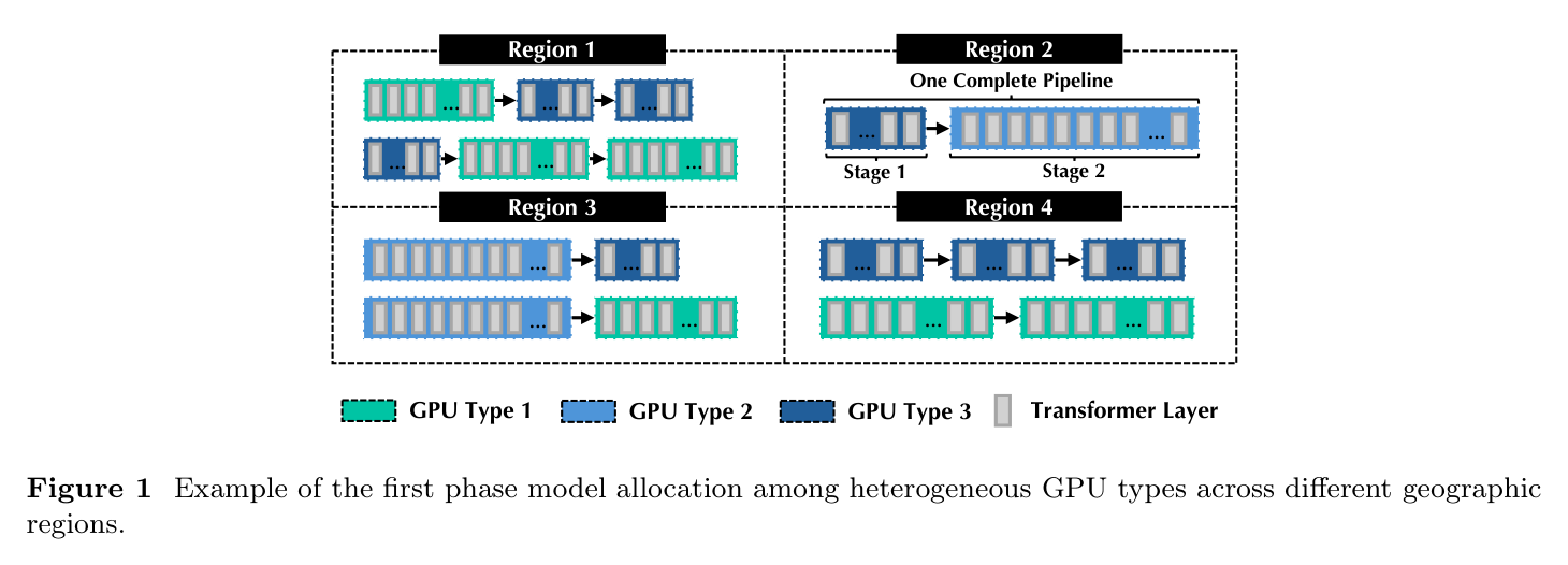
Paper's Figure 1, verbatim (caption: "Example of the first phase model allocation among heterogeneous GPU types across different geographic regions").
Four geographic regions each contain multiple pipeline replicas composed of three different GPU types. Each GPU hosts a contiguous slice of transformer layers proportional to its memory capacity. Region 2 highlights one complete pipeline spanning two stages across two GPUs. The region-based heuristic ensures no pipeline crosses regional boundaries, eliminating high-latency cross-region activation transfers on the critical path.
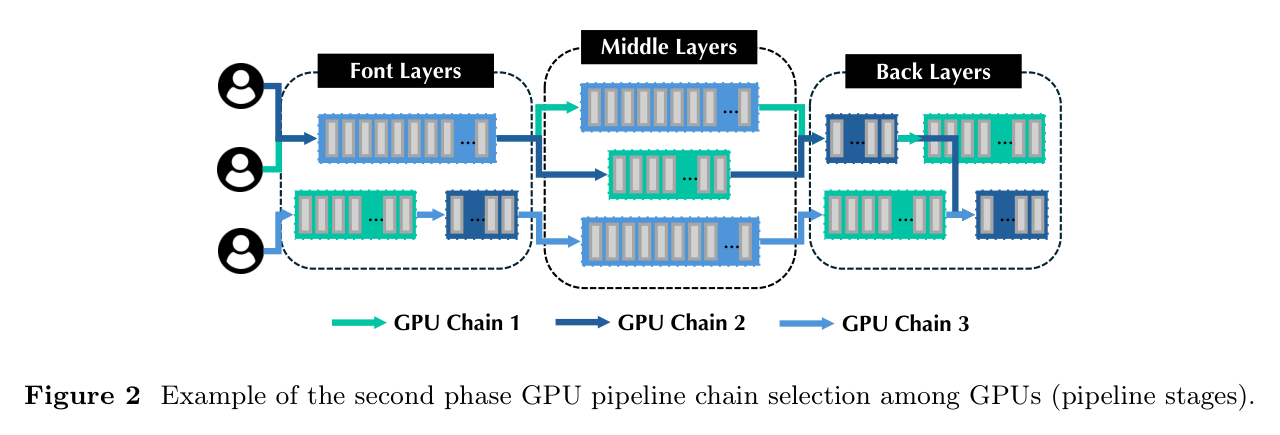
Paper's Figure 2, verbatim (caption: "Example of the second phase GPU pipeline chain selection among GPUs (pipeline stages)").
Three clients each receive a distinct GPU chain (colored arrows) traversing Front, Middle, and Back layer groups. Each chain may mix stages from different pipeline replicas — one client takes a path through certain GPUs while another takes a different path through the same layer groups. This cross-replica stitching enables load balancing: the DP selects lowest-latency paths through the DAG of available stages, naturally deflecting traffic from loaded GPUs toward idle ones.
System scope: Parallax covers both prefill and decode. Parallelism axes: request-level data parallelism (multiple replicas) + pipeline parallelism (layer partitioning within replicas). No tensor parallelism — activation communication is inter-stage only (low volume). Deployment mode: multi-node decentralized over public WAN.
§4 作者证明 #
符号表 #
| Symbol | Meaning | Domain |
|---|---|---|
| $L$ | Total transformer layers in model | $\mathbb{N}$ |
| $N$ | Number of available GPUs | $\mathbb{N}$ |
| $g_i$ | GPU $i$ in pool $\mathbf{G} = \{g_1, \dots, g_N\}$ | — |
| $c_i$ | Max layer capacity of GPU $g_i$ (VRAM-constrained) | $\mathbb{N}$ |
| $k$ | Number of pipeline replications | $\{1, \dots, k_{\max}\}$ |
| $s^{\star}(k)$ | Minimum total stages for $k$ replications | $\mathbb{N}$ |
| $r_{\mathrm{RTT}}$ | Average inter-stage hop latency (profiled) | $\mathbb{R}^+$ (s) |
| $T_{\mathrm{comp}}$ | Average per-replication compute time | $\mathbb{R}^+$ (s) |
| $F_i$ | Compute capacity (FLOPs) of GPU $g_i$ | $\mathbb{R}^+$ |
| $\lambda$ | Water-filling scaling parameter | $\mathbb{R}^+$ |
| $\tau_{g_i}$ | Profiled processing latency on GPU $g_i$ | $\mathbb{R}^+$ (s) |
| $\rho_{g_i, g_{i'}}$ | One-way RTT between GPU pair $(g_i, g_{i'})$ | $\mathbb{R}^+$ (s) |
| $\bar{R}$ | Average replicated copies per layer in DAG | $\mathbb{R}^+$ |
| $\alpha$ | Load metric weight (memory vs. compute) | $[0, 1]$, default 0.5 |
方程物理意义 #
Eq 1 — Maximum replication bound:
$$k_{\max} = \min\!\big(N,\; \lfloor \textstyle\sum_{i=1}^{N} c_i / L \rfloor\big)$$
Upper-bounds replications by the lesser of GPU count and aggregate capacity divided by model size. When total capacity barely exceeds $L$, only one replica fits regardless of GPU count.
Eq 2 — Phase 1 scoring function:
$$Z(k) = k - \frac{s^{\star}(k)/k \cdot r_{\mathrm{RTT}}}{T_{\mathrm{comp}}}$$
Effective throughput: $k$ replications minus the communication tax per replica. The ratio $r_{\mathrm{RTT}} / T_{\mathrm{comp}}$ captures how expensive each additional pipeline stage is relative to compute. In decentralized settings this ratio is large (communication-dominated), so minimizing $s^{\star}(k)/k$ (stages per replica) is critical.
Eq 3 — Phase 2 DP recurrence:
$$\mathrm{dp_2}(\ell{+}1, g_{i'}) = \min\!\big(\mathrm{dp_2}(\ell{+}1, g_{i'}),\; \mathrm{dp_2}(\ell, g_i) + \rho_{g_i, g_{i'}} + \tau_{g_{i'}}\big)$$
Standard shortest-path relaxation on the layer-indexed DAG. Node cost $\tau$ captures current compute load (updated via DHT), edge cost $\rho$ captures network overhead. The min across all predecessors finds the chain with lowest cumulative latency.
Eq 4 — Water-filling fractional allocation:
$$x_i = \min(c_i,\; \lambda F_i)$$
Allocates layers proportional to compute capacity $F_i$, capped by memory capacity $c_i$. The scaling parameter $\lambda$ (found via binary search) is the "water level" — GPUs with higher $F_i$ receive more layers until they hit their capacity ceiling. Rounded to integers via largest-remainder (Hamilton) method.
Eq 5 — Dynamic membership load metric:
$$\mathrm{Load} = \alpha \cdot \frac{\text{current\_kv\_size}}{\text{total\_cluster\_memory}} + (1 - \alpha) \cdot \frac{\text{current\_compute}}{\text{total\_cluster\_flops}}$$
Composite utilization metric balancing memory pressure (KV cache size) and compute pressure (FLOPs). Global rebalancing is triggered when the coefficient of variation of per-layer loads exceeds a configurable threshold, or when no pipeline covers all $L$ layers.
6 项检查 #
未证明的声明 #
§5 实验与数据 #
实验设置 #
延迟对比 #
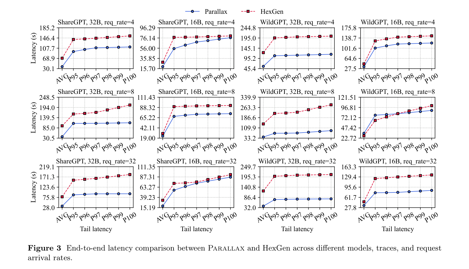
Paper's Figure 3, verbatim (caption: "End-to-end latency comparison between Parallax and HexGen across different models, traces, and request arrival rates").
A 4×3 grid of latency-percentile curves spanning two traces (ShareGPT, WildGPT), two model sizes (32B, 16B), and three request arrival rates (4, 8, 32). Parallax (blue) consistently runs below HexGen (red) across all percentiles. The gap widens at tail latencies (p97–p100) and higher request rates — the regime where communication bottlenecks and load imbalance compound. Largest improvement: WildGPT 32B at rate=32, where Parallax p99 stays under 100 s while HexGen exceeds 195 s.
吞吐对比 #
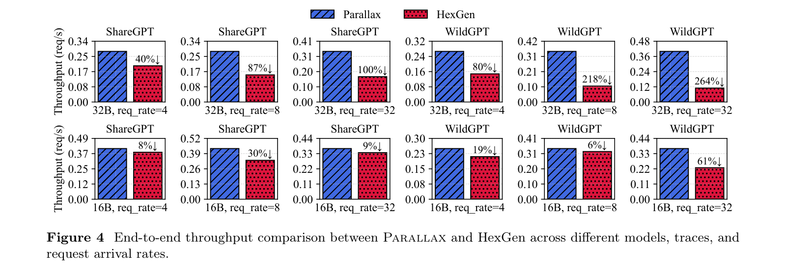
Paper's Figure 4, verbatim (caption: "End-to-end throughput comparison between Parallax and HexGen across different models, traces, and request arrival rates").
Throughput improvement percentages annotated directly on bars. The 32B model (top row) shows dramatic gains: 264% on WildGPT rate=32, 218% on WildGPT rate=8, 100% on ShareGPT rate=32. The 16B FP8 model (bottom row) shows smaller gains (6%–61%) because quantization halves model size, reducing per-stage communication volume and diminishing the scheduling advantage. This reveals Parallax's sweet spot: communication-dominated regimes where scheduling decisions have the largest impact.
调度算法可扩展性 #
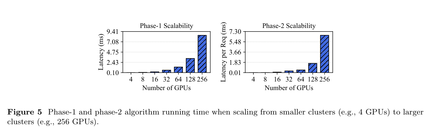
Paper's Figure 5, verbatim (caption: "Phase-1 and phase-2 algorithm running time when scaling from smaller clusters (e.g., 4 GPUs) to larger clusters (e.g., 256 GPUs)").
Phase 1 (left, one-time): 0.10 ms at 4 GPUs → 8.55 ms at 256 GPUs. Sub-10 ms even at scale enables rapid reallocation on membership changes. Phase 2 (right, per-request): 0.01 ms at 4 GPUs → 6.63 ms at 256 GPUs. Growth matches $\mathcal{O}(L\bar{R}^2)$: as cluster grows, $\bar{R}$ increases, expanding the DAG. Both overheads remain negligible relative to end-to-end inference latencies (tens to hundreds of seconds).
负载特征化 #
| Workload regime | Parallax | HexGen | Why |
|---|---|---|---|
| 32B BF16, high rate (32 req/s) | 3.6× throughput, ~2.6× p99 | Saturated | Communication-dominated; region-bounded allocation eliminates cross-region stages |
| 32B BF16, low rate (4 req/s) | ~1.4× p99 | Adequate | Less contention; scheduling helps but gap is smaller |
| 16B FP8, any rate | 6%–61% gain | Competitive | Halved model size → less communication pressure → smaller scheduling advantage |
| WildGPT vs. ShareGPT (same config) | Larger gains on WildGPT | — | Longer, more variable sequences → more load imbalance for static partitioning |
Baseline coverage gaps: only HexGen is experimentally compared. Helix (max-flow on heterogeneous GPUs, ASPLOS 2025) is cited but not benchmarked — notable given direct relevance. Petals is discussed qualitatively but also absent from experiments.
Scheduling design notes:
§6 论证链 #
| Step | Claim | Evidence | Depends on |
|---|---|---|---|
| 1 | Decentralized GPU pools suffer from compute, memory, and network heterogeneity that makes naive PP impractical | §1 qualitative analysis: cross-region latency down to hundreds of MB/s; even partitioning creates stragglers | — |
| 2 | Joint placement-and-routing is NP-hard under heterogeneity; decomposition into two DP subproblems is tractable | Claimed without proof (§3.1); tractability shown empirically via sub-10 ms overhead at 256 GPUs (Fig 5) | Step 1 |
| 3 | Phase 1 DP with region-based + latency-dominant heuristics produces compact, region-local allocations minimizing pipeline stages | Algorithm design (§3.2); region constraint eliminates cross-region edges; $Z(k)$ scoring penalizes excess stages | Step 2 |
| 4 | Phase 1's contiguous-layer, region-bounded output constrains Phase 2's DAG to small $\bar{R}$, enabling single-pass per-request chain selection in $\mathcal{O}(L\bar{R}^2)$ | Complexity analysis (§3.3); confirmed empirically: 0.01–6.63 ms/req across 4–256 GPUs (Fig 5) | Step 3 |
| 5 | Phase 2 DAG DP with live DHT metrics ($\tau$, $\rho$) naturally load-balances by deflecting requests from loaded GPUs | DHT design (§3.3): immediate $\tau$ updates on chain selection/release; shortest-path always picks currently-lowest-latency chain | Step 4 |
| 6 | Combined two-phase scheduling achieves up to 3.6× throughput and 3.2× latency improvement over HexGen | End-to-end evaluation on 7 GPUs with ShareGPT/WildGPT (§4.2, Figs 3–4); gains largest in communication-dominated regimes | Steps 3–5 |
论证弱点 #
§7 实现 cross-reference #
代码仓库: https://github.com/GradientHQ/parallax
| Component | Expected module | Paper §§ |
|---|---|---|
| Phase 1 DP + water-filling | scheduler / allocator | §3.2 |
| Phase 2 DAG DP chain selection | scheduler / router | §3.3 |
| DHT performance registry | coordination layer | §3.3 |
| Dynamic membership handler | cluster manager | §3.4 |
| Pipeline execution engine | inference runtime | §2 |
file:line 级代码分析未完成 — 仓库已公开但细粒度映射待后续补充。