Kimi Linear: An Expressive, Efficient Attention Architecture — L2 Deep Distill #

§1 TL;DR #

Kimi Linear 是首个在短/长/RL 三大场景全面超越 full attention 的混合线性注意力架构。核心模块 KDA 将 channel-wise 细粒度遗忘门与 delta rule 结合，配合 3:1 KDA-to-MLA 混合结构实现 75% KV cache 节约与 6.3× 解码加速（1M context）。48B 总参 / 3B 激活的 MoE 模型在 1.4T tokens 训练下全面超过纯 MLA baseline。

§2 Q1 / Q2 / Q3 #

Q1 痛点 #

Softmax attention 在 agent / RL test-time scaling 场景下面临二次计算复杂度和线性增长 KV cache 的双重瓶颈。现有线性注意力（含 GDN）因有限状态容量在长上下文精确检索和表达力方面受限，而 scalar decay 过于粗粒度无法精确管理 RNN 记忆。

Q2 方法 #

Kimi Delta Attention (KDA)：在 Gated DeltaNet 的 scalar $\alpha_t$ 基础上引入 per-channel diagonal decay $\text{Diag}(\boldsymbol{\alpha}_t)$，使每个特征维度拥有独立遗忘率。核心递推：

$$S_t = (I - \beta_t k_t k_t^\top) \text{Diag}(\boldsymbol{\alpha}_t) S_{t-1} + \beta_t k_t v_t^\top$$

同时将 DPLR 低秩向量 $\mathbf{a} = \mathbf{b} = \sqrt{\beta} \cdot \mathbf{k}$ 绑定到 key，使 chunkwise 算法减少 4→2 二级分块矩阵运算 + 消除 3 次额外矩阵乘法，算子速度比通用 DPLR 提升 ~100%。

混合架构采用 layerwise 3:1 KDA-to-MLA 比例，MLA 层使用 NoPE（无显式位置编码），将位置信息完全委托给 KDA 的隐式数据依赖衰减。

核心技术壁垒：将 DPLR 低秩向量绑定到 $\mathbf{k}$（$\mathbf{a}=\mathbf{b}=\sqrt{\beta}\mathbf{k}$）是 expressivity-efficiency Pareto 的关键——它保留了 fine-grained DPLR 的表达力，同时通过代数简化将 chunkwise kernel 的非 matmul FLOPs 减半，使 Tensor Core 利用率接近纯 matmul 操作。这个 constrained parameterization 是使 channel-wise gated delta rule 在实际硬件上可行的唯一已知路径。

Q3 结果 #

§3 架构 / 方法图 #

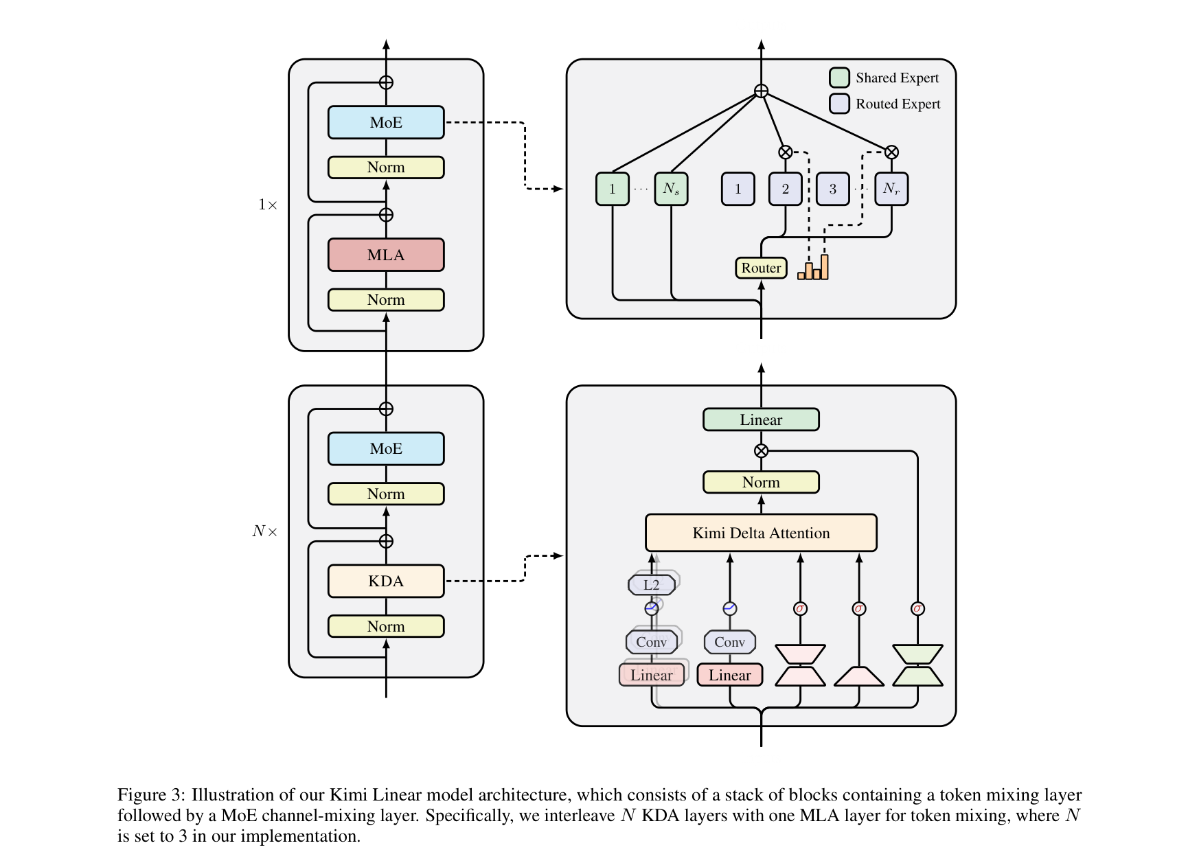
Paper's Figure 3, verbatim (caption: "Illustration of our Kimi Linear model architecture, which consists of a stack of blocks containing a token mixing layer followed by a MoE channel-mixing layer. Specifically, we interleave N KDA layers with one MLA layer for token mixing, where N is set to 3 in our implementation.").

该图展示了 Kimi Linear 的分层混合结构：每 3 个 KDA 层后接 1 个 MLA 层，所有层后接 MoE FFN（8/256 routed + 1 shared expert）。Layer 0 使用 dense FFN 保障训练稳定性。MLA 层采用 NoPE，位置编码完全由 KDA 层的 data-dependent diagonal decay 隐式提供。

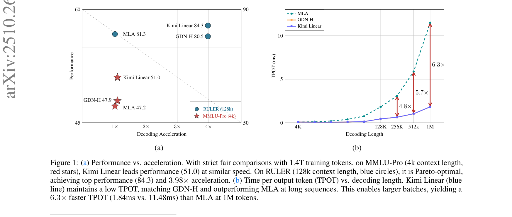
Paper's Figure 1, verbatim (caption: "(a) Performance vs. acceleration. With strict fair comparisons with 1.4T training tokens, on MMLU-Pro (4k context length, red stars), Kimi Linear leads performance (51.0) at similar speed. On RULER (128k context length, blue circles), it is Pareto-optimal, achieving top performance (84.3) and 3.98× acceleration. (b) Time per output token (TPOT) vs. decoding length.").

Figure 1a 展示 Kimi Linear 在 MMLU-Pro 和 RULER 两个维度均为 Pareto 最优；1b 展示 TPOT 随序列长度增长中 KDA 的 O(1) per-token 特性 vs MLA 的 O(n) 增长。

KDA 数据流 (from code: modeling_kimi.py:KimiDeltaAttention) #

MLA 数据流 (from code: modeling_kimi.py:KimiMLAAttention) #

代码来源：https://huggingface.co/moonshotai/Kimi-Linear-48B-A3B-Instruct/blob/main/modeling_kimi.py

§4 作者证明 #

符号表 #

方程物理意义 #

1. Eq. 1 (KDA 递推)：$S_t = (I - \beta_t k_t k_t^\top) \text{Diag}(\boldsymbol{\alpha}_t) S_{t-1} + \beta_t k_t v_t^\top$。物理含义：先按 channel 独立衰减旧记忆（$\text{Diag}(\alpha)$），再通过 Householder 变换 $(I - \beta kk^\top)$ 沿当前 key 方向投影擦除旧 value，最后写入新 $k \to v$ 映射。这是在线梯度下降 + L2 正则化的统一形式。
1. Eq. 9 (输出计算)：$O_{[t]} = (\Gamma Q) S_{[t]} + \text{Tril}((\Gamma Q)(K/\Gamma)^\top)(U - W S_{[t]})$。物理含义：输出由「查询持久记忆」（inter-chunk）和「chunk 内因果注意力」（intra-chunk，带 pseudo-value 校正）两部分组成。
1. DPLR 绑定 (§6.2)：令 $\mathbf{a} = \mathbf{b} = \sqrt{\beta} \cdot \mathbf{k}$，将通用 DPLR 的 4 自由度压缩为 2，代数上等价于 delta rule 但可利用对称性减半计算。

6 项最低检查 #

#	检查项	结果
1	维度一致性（Eq.1 $d_k \times d_v$ 输出验证）	✓ $(I - \beta kk^\top)$ 是 $d_k \times d_k$，$\text{Diag}(\alpha)$ 是 $d_k \times d_k$，$S$ 是 $d_k \times d_v$，$kv^\top$ 是 $d_k \times d_v$
2	Chunk 边界一致性（$S_{[t+1]} = S_{[t]}^C$）	✓ Eq.8 的输出作为下一 chunk 的初始状态
3	WY 表示正确性（Eq.3 与 Eq.4-5 可逆性）	✓ 论文引用 Comba [40] 证明，UT 变换通过前代消去法避免显式逆
4	DPLR 特殊化（Eq.1 → 通用 DPLR with $a=b=\sqrt{\beta}k$）	✓ §6.2 推导完整
5	数值稳定性（fine-grained decay 除法精度）	✓ §3.2 讨论了 $K/\Gamma$ 的精度问题及 KDA 绑定如何缓解
6	参数量验证（3B activated / 48B total）	✓ config.json: 256 experts × 3 × 2304×1024 + overhead ≈ 48B; 8 activated + shared ≈ 3B

Scaling-law fit #

MLA: $L = 2.3092 \times C^{-0.0536}$; Kimi Linear: $L = 2.2879 \times C^{-0.0527}$。两者 exponent 接近 (-0.054 vs -0.053)，但 KDA 的 prefactor 更低，表明相同 FLOPs 下 loss 更低。~1.16× compute efficiency 意味着 KDA 可用 86% 的计算达到相同 loss。论文坦言未对 KDA 单独调参，实际增益可能更大。

Parameter breakdown #

模块	每层参数	层数	小计
KDA attention	~39M	20	780M
MLA attention	~29M	7	203M
MoE FFN (256 experts)	~1.82B	26	47.3B
Dense FFN (layer 0)	~64M	1	64M
Embedding + LM head	377M × 2	—	754M
Total			~49B
Activated			~3.5B

与论文声称的 48B total / 3B activated 基本一致（差异来自 LayerNorm、bias、gate 权重等小项）。

KV cache capacity budget #

• MLA layer KV: compressed KV 为 $(512 + 64) = 576$ 维（kv_lora_rank + rope_dim），BF16 下每 token 1.15 KB/layer × 7 layers = 8.05 KB/token
• KDA layer: 解码时仅需 recurrent state $S \in \mathbb{R}^{128 \times 128}$ per head × 32 heads = 524K per layer（固定，不随序列增长）+ conv state 3×4096×4 = 49K/layer
• 总 KV: 7 MLA layers × 1.15 KB/token = 8.05 KB/token（vs 纯 MLA 27 layers × 1.15 = 31 KB/token → 74% 节约）

§5 实验与数据 #

Scaling Law #



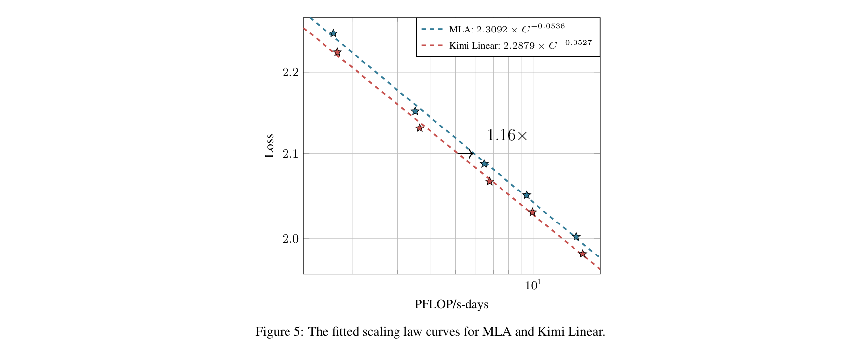
Paper's Figure 5, verbatim (caption: "The fitted scaling law curves for MLA and Kimi Linear.").

5 个模型尺度 (653M–1.7B activated) 在相同 FLOPs 下，Kimi Linear 的 loss 曲线始终低于 MLA。拟合显示 ~1.16× compute efficiency 优势。值得注意的是所有超参使用 MLA 的最优值，未针对 KDA 调优。

Synthetic Tasks #



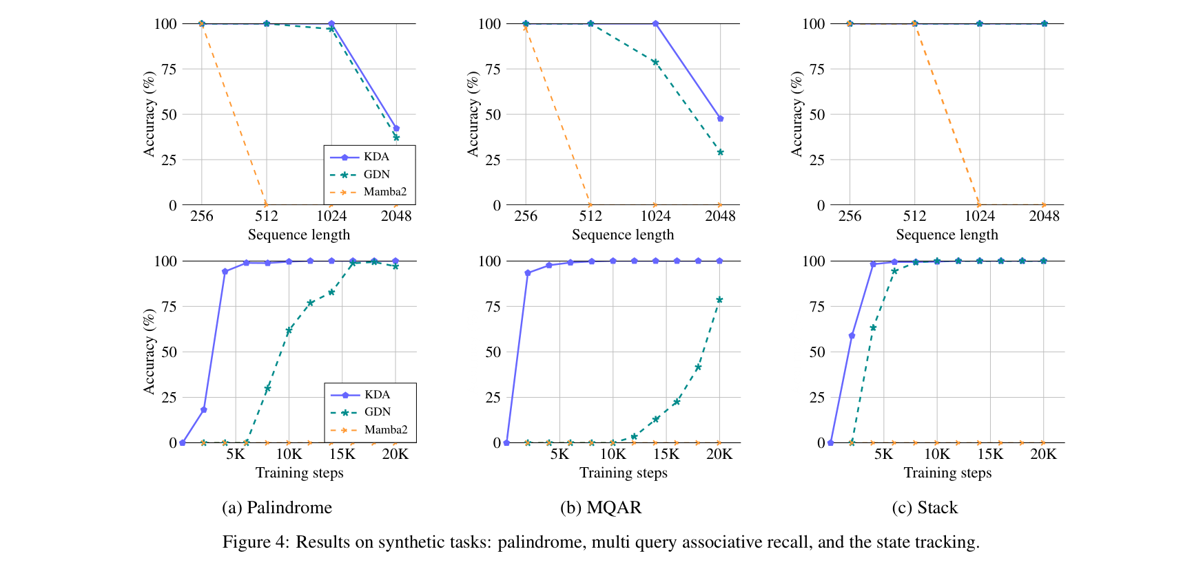
Paper's Figure 4, verbatim (caption: "Results on synthetic tasks: palindrome, multi query associative recall, and the state tracking.").

在 Palindrome（逆序复制）、MQAR（多查询关联回忆）、Stack（LIFO 栈模拟）三个任务上，KDA 在所有序列长度 (256–2048) 取得最高精度且收敛最快。Mamba2（仅乘性衰减无 delta rule）在所有任务完全失败——证明 delta rule 的自校正机制是精确检索的必要条件，而 fine-grained gating 进一步提升了记忆利用效率。

RL Post-Training #



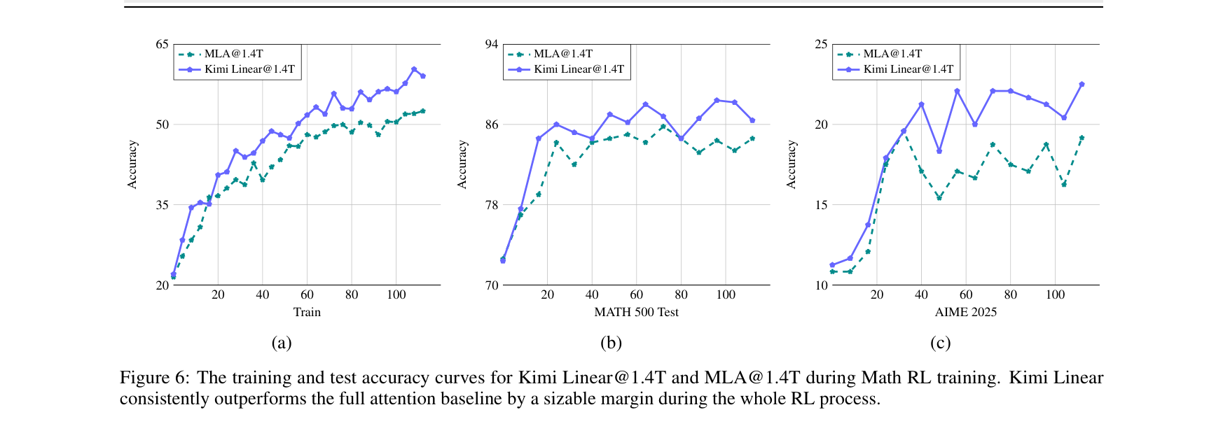
Paper's Figure 6, verbatim (caption: "The training and test accuracy curves for Kimi Linear@1.4T and MLA@1.4T during Math RL training. Kimi Linear consistently outperforms the full attention baseline by a sizable margin during the whole RL process.").

在 RLVR 数学训练中，Kimi Linear 的训练集/测试集精度增长率持续高于 MLA，AIME 2025 和 MATH500 上差距随训练逐步扩大。这表明 KDA 的高效长序列处理在 RL 长 trajectory 场景具有结构性优势。

Decoding Speed #



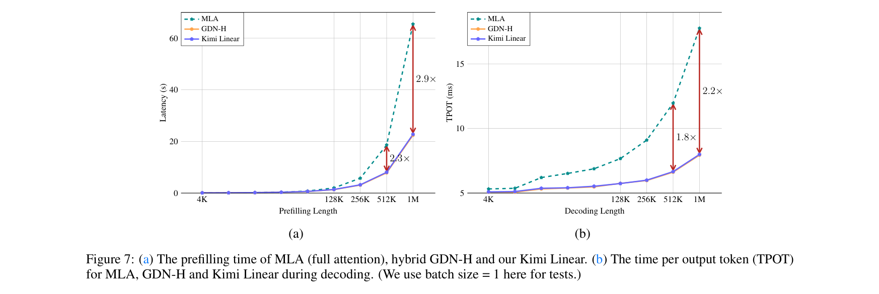
Paper's Figure 7, verbatim (caption: "(a) The prefilling time of MLA (full attention), hybrid GDN-H and our Kimi Linear. (b) The time per output token (TPOT) for MLA, GDN-H and Kimi Linear during decoding.").

Prefill 阶段 KDA 引入的额外开销相对 GDN-H 几乎可忽略。Decode 阶段 KDA/GDN-H 维持 O(1) TPOT 而 MLA 为 O(n)：在 1M tokens 处达到 6.3× 加速 (1.84ms vs 11.48ms)。

Long-Context Key Results #

Benchmark	MLA	GDN-H	Kimi Linear	Δ vs MLA
RULER (128K)	81.3	80.5	84.3	+3.0
MRCR	22.6	23.9	29.6	+7.0
HELMET-ICL	88.0	85.5	90.0	+2.0
RepoQA	63.0	63.0	68.5	+5.5
Average (8 tasks)	52.2	51.2	54.5	+2.3

GDN-H 在长上下文退化至 MLA 以下，而 Kimi Linear（仅 scalar→channel gating 差异）反而超越 MLA——证明 channel-wise decay 对长程记忆管理的临界重要性。

§6 论证链 #

Step	论据	证据	逻辑衔接
1	Softmax attention 在长序列 decode 场景有 O(n) KV cache + O(n) TPOT 瓶颈	已知事实 + Fig.7b MLA 曲线	建立痛点
2	线性注意力通过有限状态 RNN 实现 O(1) decode，但受限于记忆容量导致表达力不足	Mamba2 在合成任务完全失败 (Fig.4)	说明 vanilla 线性注意力不够
3	Delta rule 提供自校正记忆（在线梯度下降视角），但 scalar gating 对记忆管理过于粗粒度	GDN-H 在长上下文退化至 MLA 以下 (Table 5)	动机：需要 fine-grained gating
4	KDA 引入 per-channel $\text{Diag}(\boldsymbol{\alpha}_t)$ 实现每维度独立遗忘率 + 绑定 DPLR $a=b=\sqrt{\beta}k$ 保持硬件效率	Fig.2 kernel 速度 2× > DPLR; §6.2 推导	方法核心 + 效率保证
5	3:1 混合比 + NoPE MLA 是 Pareto 最优配置	Table 1 ablation: 3:1 最低 val PPL; NoPE 长上下文优势	架构设计验证
6	全流程验证：pretrain→SFT→long-context→RL 四阶段全面超过 MLA	Tables 3-5 + Fig.6	全面性证据
7	6.3× decode 加速 + 75% KV cache 节约使 1M context serving 实际可行	Fig.7b 实测 TPOT	实用性论证

§7 实现 cross-reference #

代码仓库 #

• KDA kernel: https://github.com/fla-org/flash-linear-attention/tree/main/fla/ops/kda (chunk_kda, fused_recurrent_kda)
• Model code: https://huggingface.co/moonshotai/Kimi-Linear-48B-A3B-Instruct/blob/main/modeling_kimi.py
• Config: https://huggingface.co/moonshotai/Kimi-Linear-48B-A3B-Instruct/blob/main/config.json

关键实现细节 #

1. L2Norm in kernel: use_qk_l2norm_in_kernel=True — Q、K 的 L2 归一化融合在 KDA kernel 内部（modeling_kimi.py:KimiDeltaAttention.forward），避免额外 kernel launch 且保证数值稳定性。代码中 q_conv1d 和 k_conv1d 的 activation='silu' 对应论文的 Swish 激活。
1. Gate 融合: fused_kda_gate(g, self.A_log, self.head_dim, g_bias=self.dt_bias) 将低秩 gate 投影与 log-domain decay 计算融合为单个 CUDA op（fla/ops/kda/gate.py），对应论文中 $f(\mathbf{W}_\alpha^\uparrow \mathbf{W}_\alpha^\downarrow x)$ 的高效实现。A_log 初始化为 log(Uniform(1,16))，对应 Mamba 风格的对数空间衰减参数化。
1. Recurrent vs Chunk mode 切换: mode = 'fused_recurrent' if q_len <= 64 else self.mode（modeling_kimi.py line in KimiDeltaAttention.forward）——短序列（decode）使用纯递推模式避免 chunk overhead，长序列使用 chunkwise 并行。

核心技术壁垒（§7 专段） #

DPLR $a=b=\sqrt{\beta}k$ 绑定的实现难点在于：chunkwise 算法的 WY 表示（Eq.3-5）要求在 $O(C^2 d)$ 内完成辅助向量 $w, u$ 的前代求解，而 general DPLR 的 $a \neq b$ 需要 4 组独立的二级分块矩阵运算。绑定后 $w$ 和 $u$ 共享内积 $k_i^\top \text{Diag}(\gamma^{i\to r}) k_r$，使计算量减半且 memory bandwidth 需求降低。这一简化直接决定了 KDA kernel 能否在 A100/H100 上达到接近 roofline 的效率——没有此绑定，fine-grained decay 的 chunkwise kernel 将被非 matmul 操作主导，无法超越 FlashAttention-2 的 prefill 性能。

§5 Training Recipe (model-specific) #

Stage	Goal	Data (tokens + mix)	LR schedule	Context	Techniques
Pre-training	Language modeling	1.4T tokens, shared data mix	WSD (warmup-stable-decay)	4,096	MuonClip optimizer, all models same recipe
Mid-training (context extension)	[论文未披露]	[论文未披露]	[论文未披露]	up to 1M	[论文未披露具体长上下文训练细节]
SFT	Instruction following	Curated: general knowledge + reasoning (math/code) + Chinese	[论文未披露]	[论文未披露]	Same recipe across all models
RL (RLVR)	Math reasoning	In-house math training set from [50], moderate difficulty	[论文未披露]	[论文未披露]	Same algorithm + hyperparams as MLA baseline
Quantization-aware training	[论文未披露]	[论文未披露]	[论文未披露]	—	[论文未披露]

最难复现的训练 trick: NoPE on MLA layers — 去除全注意力层的位置编码，完全依赖 KDA 层的 data-dependent decay 提供位置信息。这不是常规做法（RoPE 是 MLA 标配），需要从零开始训练以建立正确的位置-注意力耦合。论文显示 NoPE 在长上下文显著优于 RoPE 变体 (Table 5: 54.5 vs 51.8 avg)，但此设计在其他架构上是否 transferable 不明。

§8 Serving Deployment Considerations #

配置	GPU 需求	KV cache/token	Max concurrency @ 128K
BF16	~4× H100 80GB (48B params)	8 KB/token (仅 7 MLA layers)	~2,500 requests
FP8 (weights)	~2× H100	~8 KB/token (KV 仍 BF16)	~5,000 requests
[FP4 not disclosed]	[论文未披露]	—	—

• KV cache: 仅 7/27 层需要 KV cache (MLA layers)，每层 576 维 × BF16 = 1.15 KB/token/layer → 总 8.05 KB/token。对比纯 MLA (27 layers): 31 KB/token → 74% 节约
• KDA state: 固定大小 $32 \text{ heads} \times 128 \times 128 \times$ BF16 = 1 MB/layer × 20 layers = 20 MB/request（与序列长度无关）
• Prefill: KDA 层近似 O(n) (chunkwise)；MLA 层 O(n²) 但仅 7/27 → prefill 加速 ~4× (Fig.7a)
• Decode: KDA O(1)/token; MLA O(n) 但层数少 → 整体 TPOT 大幅降低
• Continuous batching: 完全兼容——KDA 的 recurrent state 是固定大小，不影响 batching scheduler。论文明确声称 "drop-in compatible with existing full-attention pipelines"
• Prefix caching: MLA 层可正常使用 prefix cache；KDA 层需要保存 conv_state + recurrent_state 作为 "prefix"，大小固定不随 prefix 长度增长

§9 Open Questions #

1. Scale saturation: KDA 的 per-channel gating 优势在更大模型（如 600B+）是否持续？更多 heads + 更大 head_dim 可能使 fine-grained control 的边际收益递减。
2. Modality transfer: KDA 的 data-dependent positional encoding 是否适用于 vision tokens（2D 结构）或 audio（连续时间序列）？NoPE 设计在 multimodal 设置中需要什么修改？
3. Hardware affinity: FP8/FP4 量化对 KDA kernel 的影响未知——chunkwise 算法中的 $K/\Gamma$ 除法对低精度格式是否产生额外数值误差？
4. RL 优势机制: 论文观察到 Kimi Linear 在 RL 中显著优于 MLA 但未解释机制。猜测：KDA 的 O(1) decode 允许更长 rollout 而不触发 OOM，或 fixed-size state 提供更稳定的梯度信号？
5. GDN-H 长上下文退化: scalar gate 为何在短上下文表现正常但长上下文退化？可能是 scalar decay 无法为不同频率的信息分配不同保留时间，导致高频细节与低频语义互相干扰。

Appendix: 模型架构图（代码驱动） #

代码来源：https://huggingface.co/moonshotai/Kimi-Linear-48B-A3B-Instruct/blob/main/modeling_kimi.py

A1: Top-Level #

flowchart TB subgraph Embedding EMB["nn.Embedding(163840, 2304)"] end subgraph Blocks["27 × KimiDecoderLayer"] L0["Layer 0: MLA + Dense MLP"] L1["Layer 1: KDA + MoE(8/256+1shared)"] L2["Layer 2: KDA + MoE"] L3["Layer 3: KDA + MoE"] L4["Layer 4: MLA + MoE"] LDOTS["... (3:1 pattern repeats)"] L26["Layer 26: KDA + MoE"] end subgraph Head NORM["RMSNorm(2304)"] LMH["lm_head: Linear(2304→163840)"] end EMB --> L0 --> L1 --> L2 --> L3 --> L4 --> LDOTS --> L26 L26 --> NORM --> LMH

A2: Single Transformer Block #

flowchart TB IN["hidden_states"] --> RES1["residual = x"] RES1 --> LN1["input_layernorm: RMSNorm(2304)"] LN1 --> ATTN["self_attn (KDA or MLA)"] ATTN --> ADD1["x = residual + attn_out"] ADD1 --> RES2["residual = x"] RES2 --> LN2["post_attention_layernorm: RMSNorm(2304)"] LN2 --> FFN["MoE: gate(256) → top-8 experts(2304→1024→2304) + shared_expert(2304→1024→2304)"] FFN --> ADD2["x = residual + ffn_out"] ADD2 --> OUT["output"]

A3: KDA Attention Variant #

见 §3 中的 KDA 数据流 Mermaid 图。关键维度：

• Q/K: 32 heads × 128 dim = 4096 total
• V: 32 heads × 128 dim = 4096 total
• Gate (α): low-rank 2304→128→4096 + fused with A_log (log-space decay)
• Beta: 2304→32 (per-head scalar)
• Output gate: low-rank 2304→128→4096 + FusedRMSNormGated(sigmoid)
• Recurrent state: $S \in \mathbb{R}^{32 \times 128 \times 128}$ (BF16, 固定 1MB/layer)

A4: MLA Attention Variant (辅 Attention) #

见 §3 中的 MLA 数据流 Mermaid 图。关键维度（from config.json）：

• Q: 32 heads × (128 nope + 64 rope) = 6144
• KV latent: kv_lora_rank=512, expanded to 32×(128+128)=8192
• k_rope: 64 dim (shared across heads, MQA-style)
• NoPE: mla_use_nope=true — 不对 Q/K 应用 RoPE（尽管 config 中保留了 rope 参数兼容性）
• KV cache per token: 576 × BF16 = 1.15 KB/layer

A5: MoE Gate/Routing #

flowchart LR X["x ∈ ℝ^2304"] --> GATE["Linear(2304→256) → sigmoid"] GATE --> BIAS["+e_score_correction_bias"] BIAS --> GROUP["group_scores (topk_group=1)"] GROUP --> TOPK["top-8 experts selected"] TOPK --> RENORM["renormalize weights × routed_scaling_factor=2.446"] RENORM --> DISPATCH["dispatch to 8 experts"] DISPATCH --> AGG["weighted sum + shared_expert output"]

A6: Residual Connection #

N/A — 模型使用标准 Pre-Norm residual connection（x = residual + layer(norm(x))），无 mHC / Highway / DenseNet 变体。

代码-图对照表 #

代码构件	对应图	关键实现细节
KimiDeltaAttention	A3	chunk_kda/fused_recurrent_kda 切换阈值 q_len=64
KimiMLAAttention	A4	use_nope=True 跳过 RoPE；q_lora_rank=None（无 Q 压缩）
KimiSparseMoeBlock	A5	sigmoid gating + bias correction + group topk
KimiDecoderLayer	A2	is_kda_layer() 决定 attention 类型
KimiLinearModel	A1	first_k_dense_replace=1 → layer 0 无 MoE
KimiDynamicCache	—	conv_states + recurrent_states (KDA) / key_cache + value_cache (MLA)
FusedRMSNormGated	A3 output	sigmoid gate 融合到 RMSNorm 内
ShortConvolution(kernel=4, silu)	A3 input	depthwise conv on Q/K/V 各自独立