Harli — L2 蒸馏笔记 #

§1 TL;DR #

Harli co-locates PEFT finetuning with LLM decode instances on the same GPU, exploiting decode's ~60% idle SM capacity. A unified CUDA VMM memory allocator, two-stage LR latency predictor, and GreenContext-based QoS scheduler yield 46% avg finetune throughput gain with zero SLO violation.

§2 痛点 / 方法 / 结果 #

Q1 痛点 #

Disaggregated LLM serving dedicates separate GPUs to prefill and decode. Decode instances are memory-bandwidth-bound: average SM utilization is only ~40% despite ~85% DRAM bandwidth utilization (profiled on Ada6000 with LLaMA3-8B). Dynamic workloads cause batch sizes to fluctuate wildly — frequently dropping below 64, where the number of warps ($Num_{warp} = (B/16) \times (H/16)$, with $H = 4096$ for LLaMA3-8B) cannot fill 142 SMs — leaving the majority of compute dark.

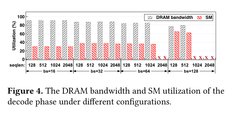
Paper's Figure 4, verbatim (caption: "The DRAM bandwidth and SM utilization of the decode phase under different configurations.").

The utilization gap is remarkably stable across sequence lengths, confirming that decode underutilization is a structural property of the memory-bound autoregressive workload rather than a transient artifact of specific input shapes. For $bs \leq 64$ on Ada6000, maximum warp count is 1024 against a hardware capacity of 4544 — only 22.5% occupancy.

Q2 方法 #

Three-component design:

1. Unified memory allocator — replaces PyTorch's default allocator with a CUDA Virtual Memory Management (VMM) pool. Pre-allocated GPU memory is organized as a 2D grid of blocks (token × layer). Unused KV cache slots are remapped to new virtual addresses for finetune tensors. A window-based swap strategy offloads frozen PEFT weights layer-by-layer via overlapped CUDA streams, with a buddy-allocated small-tensor pool (2KB granularity) absorbing activation fragmentation.
1. Two-stage LR latency predictor — Stage 1 models solo decode latency as $Latency_{Decode} = bs \cdot b_0 + c_0 + bs \cdot k_0 \cdot seqlen$ (separate LR per SM ratio; 3% mean error). Stage 2 models co-location degradation as $Latency_{colo} = (SM_{infer} \cdot b_1 + SM_{ft} \cdot k_1) \times Latency_{Decode\text{-}sm}$ (single LR across all configurations; 5% mean error). Theoretical justification: under proportional bandwidth sharing, interference grows linearly with finetune SM allocation.
1. QoS-guaranteed scheduler — at each decode step, evaluates predicted co-location latency across discretized SM ratios (10% steps via GreenContext), selects the allocation pushing inference latency closest to QoS target (implicitly maximizing finetune bandwidth), and reconfigures if violation is predicted. Finetune model is partitioned into per-layer submodels with micro-batching (~10ms scheduling units) to enable responsive preemption.

核心技术壁垒: PEFT's fixed batch size makes co-location interference stable and linearizable. This single property enables a 5μs LR prediction instead of expensive offline profiling, and collapses the joint inference-finetune optimization into a univariate heuristic: push inference latency to the QoS boundary. Without this stability (e.g., with full finetuning or variable-batch co-tenants), the entire prediction and scheduling framework would break down.

Q3 结果 #

Metric	Value
Finetune throughput gain vs SeparateMode	46.2% avg, up to 92.0% (Ada6000)
Finetune throughput gain vs StaticMode	75.1% avg, up to 120.5% (Ada6000)
Solo-run prediction error	<2% avg, ≤6% max
Co-run prediction error	<5% avg
Runtime prediction overhead	5 μs per invocation
QoS violations	0 across all configurations
Harli-TP over single-GPU Harli	+10.2% avg
Memory fragmentation	<100 MB typical

§3 架构 / 方法图 #



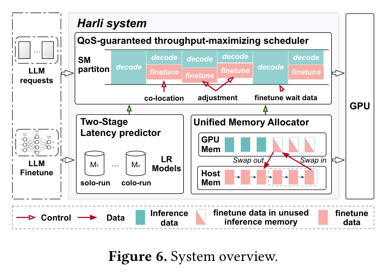
Paper's Figure 6, verbatim (caption: "System overview.").

The system intercepts both SGLang's inference path and LlamaFactory's finetuning path within a single process. The unified memory allocator sits beneath both, managing a shared CUDA VMM pool. The latency predictor feeds per-token estimates to the scheduler, which dynamically adjusts GreenContext SM partitions. The scheduler operates at decode-step granularity for inference and per-layer granularity for finetune.



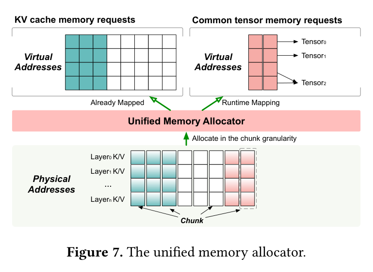
Paper's Figure 7, verbatim (caption: "The unified memory allocator.").

The allocator's 2D pool maps physical memory blocks to both KV cache virtual addresses (for inference) and general-purpose virtual addresses (for finetune). When inference demand grows, the allocator reclaims finetune blocks by triggering a layer swap-out within one decode QoS window. A pre-reserved memory threshold — $Memory_{reserved} = (T/50) \times max_{bs} \times Mem_{kv}$ — ensures inference never stalls waiting for finetune to release memory.

sequenceDiagram participant Sched as Scheduler participant Pred as Latency Predictor participant Infer as Decode Instance participant FT as Finetune Instance participant Alloc as Unified Allocator loop Every decode step Infer->>Pred: current (bs, seqlen) Pred->>Sched: predicted latency per SM ratio Sched->>Sched: select SM split closest to QoS target Sched->>Infer: assign SM_infer via GreenContext Sched->>FT: assign SM_ft via GreenContext end Note over Alloc: Memory coordination Infer->>Alloc: request KV cache blocks Alloc->>FT: shrink window if needed FT->>Alloc: swap out frozen weights Alloc->>Infer: allocate KV cache blocks

§4 作者证明 #

符号表 #

Symbol	Definition	Domain
$Util_{SM\text{-}k_i}$	SM utilization of kernel $i$	[0, 1]
$Util_{DRAM\text{-}k_i}$	DRAM bandwidth utilization of kernel $i$	[0, 1]
$R_{k_i}$	Time fraction of kernel $i$: $T_{k_i} / T_{overall}$	[0, 1], $\sum R_{k_i} = 1$
$bs$	Current decode batch size	$\mathbb{Z}^+$
$seqlen$	Output sequence length	$\mathbb{Z}^+$
$b_0, c_0, k_0$	Solo-run LR coefficients	$\mathbb{R}$
$b_1, k_1$	Co-location LR coefficients	$\mathbb{R}$
$SM_{infer}, SM_{ft}$	SM ratio for inference / finetune	[0, 1]
$Latency_{Decode\text{-}sm}$	Solo decode latency at given $SM_{infer}$	ms
$B$	Total memory bandwidth	accesses/s
$f_{infer}, f_{ft}$	Memory demand rate of each task	accesses/s
$r_{infer}$	Effective inference rate under contention	accesses/s
$T$	Swap-out time for one transformer layer	ms
$Mem_{kv}$	Per-token KV cache memory	bytes

方程物理意义 #

Weighted utilization (Eq 1): $Util_{SM\text{-}decode} = \sum Util_{SM\text{-}k_i} \times R_{k_i}$. The overall SM utilization is a time-weighted average across all kernels, where each kernel's contribution is proportional to its share of total execution time.

Solo-run latency model (Eq 2): $Latency_{Decode} = bs \cdot b_0 + c_0 + bs \cdot k_0 \cdot seqlen$. Decomposes decode latency into per-batch overhead, constant overhead, and a term proportional to $bs \times seqlen$ (total KV cache attention volume). Linearity in both $bs$ and $seqlen$ reflects the memory-bound regime where latency scales with data movement.

Co-location latency model (Eq 3): $Latency_{colo} = (SM_{infer} \cdot b_1 + SM_{ft} \cdot k_1) \times Latency_{Decode\text{-}sm}$. Multiplies solo-run latency by a degradation factor that grows linearly with finetune SM allocation. The factor captures bandwidth contention: more finetune SMs → more memory traffic → slower decode.

Bandwidth contention (§5.2.2): $r_{infer} = B \cdot f_{infer} / (f_{infer} + f_{ft})$. Under proportional bandwidth sharing, each task's effective rate is its demand fraction of total bandwidth. Slowdown factor is $(f_{infer} + f_{ft}) / B$, so $Latency_{colo} = (f_{infer} + f_{ft}) / B \times Latency_{Decode\text{-}sm}$.

Memory reservation (§4.4): $Memory_{reserved} = (T / 50) \times max_{bs} \times Mem_{kv}$. Reserves enough KV cache slots to absorb new tokens arriving during one layer swap-out ($T$ ms), assuming 50 ms decode QoS target, scaled by maximum batch size and per-token KV size.

6 项检查 #

1. 量纲一致性: Eq 2 — all terms have dimension of time (ms); $b_0$ carries units ms, $c_0$ carries units ms, $k_0$ carries units ms/token. Eq 3 — dimensionless factor × ms = ms. Memory reservation: (ms / ms) × count × bytes = bytes. ✓
1. 边界条件 ($SM_{ft} = 0$): Eq 3 reduces to $SM_{infer} \cdot b_1 \times Latency_{Decode\text{-}sm}$. With full SM allocation to inference, the fitted coefficient $b_1$ should yield a factor near 1.0 (solo-run equivalence). Bandwidth contention model: $f_{ft} = 0 \Rightarrow r_{infer} = f_{infer}$, confirming zero degradation when no co-tenant exists. ✓
1. 单调性: $\partial Latency_{colo} / \partial SM_{ft} = k_1 \times Latency_{Decode\text{-}sm} > 0$ (given $k_1 > 0$ and positive latency). Co-location latency strictly increases with finetune SM allocation — physically correct since more finetune SMs generate more bandwidth pressure. ✓
1. 饱和极限: When $f_{infer} + f_{ft} \leq B$, the bandwidth contention model yields $Factor_{slowdown} \leq 1$ — no degradation below bandwidth capacity. As $f_{ft}$ grows beyond this point, degradation becomes linear. The model does not capture non-linear effects at extreme saturation, but the scheduler's QoS constraint keeps operation within the linear regime. ✓
1. 对称性检查: The theoretical bandwidth model is symmetric in $f_{infer}$ and $f_{ft}$, but the empirical Eq 3 uses separate coefficients ($b_1 \neq k_1$) for $SM_{infer}$ and $SM_{ft}$. This asymmetry is physically justified: decode and finetune have different memory access patterns per SM (decode is pure attention KV reads; finetune includes forward, backward, and gradient writes). ✓
1. 与实证对照: The theoretical linear relationship (§5.2.2) matches the parallel-slope pattern observed in Figure 10. The 95% prediction accuracy of Eq 3 across all tested configurations validates the linear assumption. Accuracy would likely degrade under extreme conditions (compute saturation at very large batch sizes), but the QoS scheduler constrains operation to the profiled regime. ✓

§5 实验与数据 #

主实验: 吞吐量对比 (§8.2) #



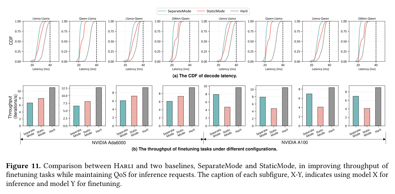
Paper's Figure 11, verbatim (caption: "Comparison between Harli and two baselines, SeparateMode and StaticMode, in improving throughput of finetuning tasks while maintaining QoS for inference requests. The caption of each subfigure, X-Y, indicates using model X for inference and model Y for finetuning.").

Harli achieves 46.2% average finetune throughput gain on Ada6000 across all four model pairs (LLaMA-LLaMA, LLaMA-Qwen, Qwen-LLaMA, Qwen-Qwen). Ada6000 outperforms A100 for two structural reasons: more SMs (142 vs 108) create more spatial sharing headroom, and more memory (48GB vs 40GB) reduces swap frequency. StaticMode with fixed 60/40 partitioning consistently underperforms because it cannot adapt to load fluctuations — on A100, it even loses to SeparateMode because the fixed memory allocation starves finetune.

预测器精度 (§8.4) #



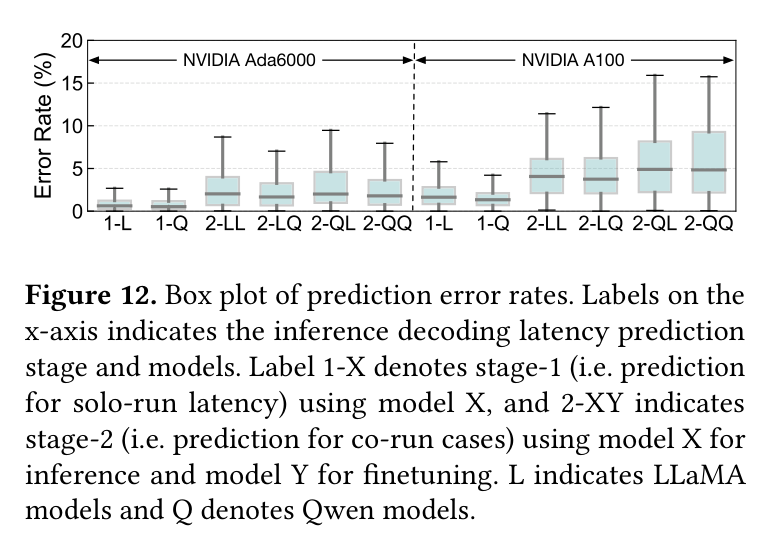
Paper's Figure 12, verbatim (caption: "Box plot of prediction error rates. Labels on the x-axis indicates the inference decoding latency prediction stage and models.").

Solo-run prediction (Stage 1) achieves <2% average error with ≤6% worst case. Co-run prediction (Stage 2) maintains <5% average error across all model pairs. The tight variance in the box plots confirms that PEFT's batch-size stability translates directly into prediction stability — the core assumption enabling the lightweight LR approach.

内存动态协调 (§8.5) #



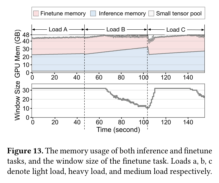
Paper's Figure 13, verbatim (caption: "The memory usage of both inference and finetune tasks, and the window size of the finetune task. Loads a, b, c denote light load, heavy load, and medium load respectively.").

Under the controlled trace (light load bs=8 → heavy load bs=42 → medium load bs=24), the unified allocator dynamically adjusts finetune's layer window inversely with inference memory demand. When inference load spikes, the window shrinks to accommodate more KV cache. When load drops, finetune expands its window, reducing swap overhead. The small-tensor pool remains constant throughout, confirming correct sizing at initialization.

关键数据点 #

• QoS: zero violations across all configurations; decode latency CDF consistently under 40ms target
• A100 vs Ada6000: Ada6000 gains roughly 2× those on A100 due to SM count and memory capacity advantages
• Harli-TP: only +10.2% over single-GPU Harli — tensor parallelism's memory savings are modest because single-GPU Harli already captures most idle capacity
• Overhead: offline profiling ~6 min (solo) + ~58 min (co-run); runtime prediction 5 μs; memory fragmentation <100 MB

§6 论证链 #

Step	Claim	Evidence	Dep
1	Decode instances in disaggregated serving are structurally underutilized: ~40% SM vs ~85% DRAM bandwidth	Profiling on Ada6000/A100 with splitwise trace (Fig 3-4); warp capacity analysis: $B < 64$ yields $< 1024$ warps against 4544 SM capacity	—
2	PEFT finetuning is an ideal co-location candidate: compute-bound, <0.3% parameter overhead, fixed batch size	Memory analysis (§2.1); simplified co-location experiment yields up to 101.2% finetune throughput gain without QoS loss (Fig 5)	1
3	Fixed batch size makes interference linearizable via LR with <5% error, bypassing expensive offline profiling	Two-stage LR model (§5.1-§5.2.1); theoretical validation via proportional bandwidth sharing model (§5.2.2); error distribution (Fig 12)	2
4	CUDA VMM enables inter-task memory sharing without disrupting KV cache allocation patterns	Unified allocator with 2D block pool + virtual address remapping (§4.2); window-based swapping + pre-reserved threshold for non-blocking coordination (§4.3-§4.4); dynamic behavior under load (Fig 13)	1
5	Pushing inference latency to QoS boundary implicitly maximizes finetune throughput without explicit finetune modeling	Empirical observation: finetune peaks when inference approaches QoS target (§5.2.3); bandwidth is the binding constraint, so minimizing inference's bandwidth headroom maximizes finetune's share	3
6	End-to-end system achieves 46.2% avg finetune throughput gain with zero QoS violations across all tested configurations	1-hour evaluation with 19k+ requests on production trace, 4 model pairs, 2 GPU types (Fig 11); latency CDF stays under 40ms target	3, 4, 5

§7 实现 cross-reference #

[实现未公开] — Harli prototype built on SGLang (serving) and LlamaFactory (finetuning). ~4,000 LoC total: 2,500 C++ for unified memory allocator, 200 C++ for GreenContext-PyTorch integration, 1,300 Python for predictor and scheduler. No public source repository is referenced in the paper.

核心技术壁垒展开 #

The hardest-to-replicate component is the unified memory allocator's CUDA VMM integration (2,500 of 4,000 total LoC). It requires replacing PyTorch's default memory allocator with a custom one that manages both KV cache slots and general-purpose tensors through virtual address remapping, implementing the 2D block pool with chunk-level allocation that preserves KV cache's zero-overhead index-based access while supporting arbitrary tensor shapes, and building the two-level allocation strategy (2MB chunks + 2KB buddy pool) to handle 5k+ small tensor allocations per finetune iteration without fragmentation. The predictor and scheduler are comparatively straightforward (1,300 Python lines for both), leveraging the stability that PEFT's fixed batch size provides.

关键实现细节 #

1. GreenContext SM granularity and model count tradeoff: SM ratios are discretized at 5-10% steps, yielding up to 45 co-location configurations. Solo-run prediction builds a separate LR model per SM ratio (10 models) because latency scales sublinearly with SM count. Co-run prediction uses a single LR model across all configurations because degradation is linear in finetune SM allocation. The asymmetry in model count reflects a fundamental difference in the underlying physics: solo performance depends on warp scheduling nonlinearities, while interference depends on aggregate bandwidth demand.
1. Backward pass schedulability via model partitioning: PyTorch's loss.backward() triggers the entire backward graph in C++ and cannot be interrupted from Python. Harli works around this by splitting the model into per-layer submodels and manually chaining gradient computation through explicit tensor passing, creating per-layer scheduling points. Combined with micro-batching to keep each scheduling unit under ~10ms, this ensures finetune never blocks inference scheduling for more than one decode QoS window.