Draft-Conditioned Constrained Decoding for Structured Generation in LLMs
Draft-Conditioned Constrained Decoding for Structured Generation in LLMs — L2 #
1. TL;DR #
Constrained decoding masks+renormalizes each step; when the base model puts little mass on schema tokens, this is a reverse-KL projection with a large "projection tax" that steers toward valid-but-wrong outputs. DCCD first generates an unconstrained draft, then constrains conditioned on it — raising feasible mass, cutting distortion, keeping exact validity. +24pp on GSM8K (1B: 15.2%→39.0%).
2. 痛点 / 方法 / 结果 (Q1 / Q2 / Q3) #
Q1 — 痛点. Hard structural constraints (JSON schema, CFG, tool-call signatures) are non-negotiable in agentic/tool pipelines: one bad brace breaks downstream execution. Standard constrained decoding (CD) guarantees validity by masking invalid tokens and renormalizing at each step — but this is not a passive filter. When the base model assigns low probability to the schema-forced token (e.g. {, ", a field name), renormalization is a large perturbation. Repeated across many low-entropy formatting steps, this induces a trajectory bias toward prefixes that are easy to keep valid, even when they correspond to a wrong solution. Prior work documents 10–30% degradation vs unconstrained generation.
Q2 — 方法. DCCD = training-free two-step inference that decouples semantic planning from structural enforcement. Step 1: draft $y \sim p_{\mathrm{draft}}(\cdot\mid x)$ — free-form reasoning/plan, not required to be valid. Step 2: constrained-decode the final structured output conditioned on $(x,y)$, masking on the same valid-next-token set $A(h_t)$ but scoring with the draft-conditioned distribution $p_2(\cdot\mid x,y,z_{
- 核心技术壁垒: the insight that feasible mass $\alpha(h_t)$ is not fixed at inference — while $\pi_\theta$ and the valid set $A(h_t)$ are fixed, the conditioning context is free, so appending a draft $d$ moves probability onto schema tokens ($\alpha(h_t;d)\gg\alpha(h_t)$) and shrinks the per-step $\mathrm{KL}=\log\frac1{\alpha}$ without relaxing any constraint. This reframes the quality-validity tradeoff as an artifact of how constraints are enforced, not an intrinsic cost.
Q3 — 结果. Across GSM8K, GSM-Symbolic, MATH500, FOLIO and 1B–14B models, DCCD gives the best aggregated strict accuracy at every scale, largest relative gains for small models (Qwen2.5-1.5B 22.8→36.8 avg). Test-time compute converts to accuracy better than CD (GSM8K 78→83 vs CD 64→73 as $n$: 1→13). ~78–80.5% win rate on non-verifiable summarization. +39% response confidence (0.527 vs 0.393).
3. 架构 / 方法图 #
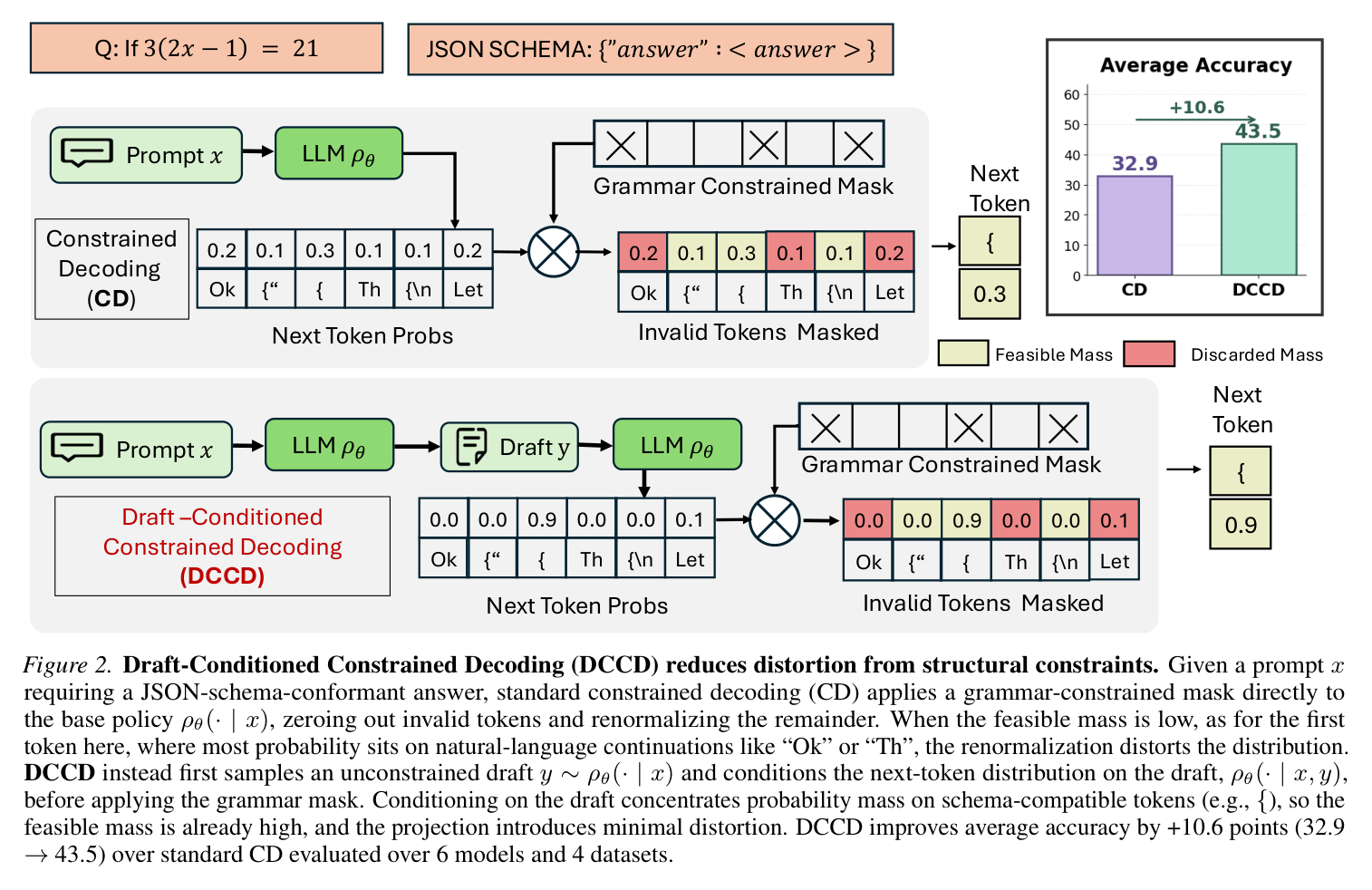
Paper's Figure 2, verbatim (caption: "Draft-Conditioned Constrained Decoding (DCCD) reduces distortion from structural constraints... DCCD instead first samples an unconstrained draft $y\sim\rho_\theta(\cdot\mid x)$ and conditions the next-token distribution on the draft... before applying the grammar mask.").
Top row (CD): the base policy's next-token probs (e.g. mass on natural-language Ok, Th) get the grammar mask applied directly — the schema token { has only 0.3 mass, so masking+renormalization heavily distorts. Bottom row (DCCD): after conditioning on draft $y$, the same { token now carries 0.9 mass, so applying the identical mask barely perturbs the distribution. The inset bar shows the net effect: +10.6 avg accuracy (32.9→43.5) across 6 models × 4 datasets. Notice the mask is identical in both rows — DCCD changes only the distribution being projected, never the constraint.
The two-stage control flow (draft model → projector with masking) is a sequence, not a per-block architecture:
The draft never enters the validity check: the mask keys on $A(h_t)$ where $h_t=(x,z_{
4. 作者证明 #
Notation table.
| Symbol | Meaning |
|---|---|
| $x,\ z_{1:T},\ V$ | prompt, output token seq (len $T$), vocabulary |
| $\pi_\theta,\ \rho_\theta$ | base LM per-step / induced sequence distribution |
$h_t \triangleq (x,z_{| decoding state (constraint keys on this) | |
| $L(x)\subseteq V^*$ | set of structurally valid sequences |
| $A(h_t)$ | valid-next-token set (tokens with ≥1 valid completion) |
| $\alpha(h_t)=\sum_{a\in A(h_t)}\pi_\theta(a\mid h_t)$ | feasible mass |
| $q,\ \rho_q$ | constrained per-step / sequence distribution |
| $d,\ y$ | auxiliary draft context / instantiated draft |
| $\alpha(\tilde h_t)=\sum_{a\in A(h_t)}p_2(a\mid \tilde h_t)$ | draft-conditioned feasible mass, $\tilde h_t=(x,y,z_{ |
| $\bar U$ | validity-gated utility $U\cdot\mathbb{I}[z\in L(x)]$ |
方程物理意义. Base factorization $\rho_\theta(z_{1:T}\mid x)=\prod_t \pi_\theta(z_t\mid h_t)$ (Eq.1). CD reweights: $q(z_t\mid h_t)=\pi_\theta(z_t\mid h_t)\mathbb{I}[z_t\in A(h_t)]/\alpha(h_t)$ (Eq.4). The per-step distortion is exactly $\mathrm{KL}(q\|\pi_\theta)=\log\frac1{\alpha(h_t)}$ (Eq.5) — small feasible mass ⇒ large distortion. Summed over the trajectory this is an additive projection tax $\mathrm{KL}(\rho_q\|\rho_\theta)=\mathbb{E}_{z\sim\rho_q}\big[\sum_t\log\frac1{\alpha(h_t)}\big]$. Geometrically, $q(\cdot\mid h_t)=\arg\min_{p\in\Delta_{A(h_t)}}\mathrm{KL}(p\|\pi_\theta)$ (Eq.7): CD = repeated reverse-KL projection onto the valid simplex. Even among valid strings, $\rho_q(z\mid x)=\rho_\theta(z\mid x)/\prod_t\alpha(h_t)$ (Eq.8) — a prefix-dependent reweighting that favors "easy-to-project" prefixes. DCCD keeps the mask on $A(h_t)$ but swaps $\pi_\theta$ for the draft-conditioned $p_2$ (Eq.14), raising $\alpha(\tilde h_t)$ (Eq.15). Appendix A closes the loop: for validity-gated utility, the utility gap between any $P,Q$ is bounded $\le \mathrm{TV}(P,Q)\le\sqrt{\tfrac12\mathrm{KL}(P\|Q)}$ (Eq.17, Pinsker). With $P=\rho_q,\ Q=\rho_\theta$ and the projection-tax identity (Eq.18), raising $\alpha(h_t)$ shrinks the KL and tightens the worst-case accuracy loss.
6 minimum checks.
- Eq.5 consistency: $\mathrm{KL}(q\|\pi)=\sum_a q(a)\log\frac{q(a)}{\pi(a)}=\sum_{a\in A}q(a)\log\frac1{\alpha}=\log\frac1\alpha$ since $q$ is supported on $A$ — ✓ (uses $q(a)=\pi(a)/\alpha$).
- Eq.8 telescoping: $\prod_t \pi_\theta(z_t\mid h_t)/\alpha(h_t)=\rho_\theta(z\mid x)/\prod_t\alpha(h_t)$ — ✓ numerator is exactly the base factorization (Eq.1).
- Projection-tax sign: $\alpha\in(0,1]\Rightarrow\log\frac1\alpha\ge0$, so the tax is nonnegative and monotone in $-\log\alpha$ — ✓ physically a "cost".
- Feasible-mass monotonicity claim (Eq.11): $\pi_\theta(s_t\mid h_t,d)\gg\pi_\theta(s_t\mid h_t)\Rightarrow\alpha(h_t;d)\gg\alpha(h_t)$ — holds when the extra mass lands on tokens inside $A(h_t)$; the paper asserts drafts do this for formatting tokens, empirically confirmed by Fig.3 (per-token $\alpha$ rises 0.34→0.85, 0.53→0.95).
- Pinsker direction (Eq.17): TV bound uses $\mathrm{KL}(P\|Q)$ with $Q=\rho_\theta$ high-utility reference; note this bounds loss relative to base, not absolute optimality — the base model itself must be competent. Consistent, but the guarantee is only as good as $\rho_\theta$'s utility.
- Best-of-$K$ selector (Alg.1): $k^\star=\arg\max_k \sum_t\log\alpha^{(k)}_t$ maximizes cumulative feasible mass ⇔ minimizes the projection tax of the realized trajectory — a coherent surrogate, but it selects for low distortion, not directly for correctness (see §6 step 4).
- The mask keys only on the final-output prefix $A(h_t)=A(x,z_{
- The selection signal is the distortion surrogate itself: best-of-$K$ ranks drafts by cumulative log feasible mass $\sum_t\log\alpha^{(k)}_t$ (Alg.1), requiring no external verifier — the draft that made the constraint least distortive is chosen. The paper notes this is swappable (log-likelihood, verifier, judge, majority vote).
- No new hardware minimum vs the base models: DCCD is training-free and reuses the same LMs; Table 1 models span Llama-3.2-1B → Qwen2.5-14B, all standard-precision instruction-tuned checkpoints.
- Latency cost is the draft pass: Step 1 generates $K$ full drafts, Step 2 runs one constrained projection on the selected draft. Total decode cost ≈ $K\times$ draft length + 1 constrained pass — the param-efficiency win (Fig.6) is per-parameter accuracy, not per-FLOP latency; best-of-$K$ trades compute for accuracy (Fig.7).
- Prefix-caching friendly: the projector conditions on $(x,y)$; the draft $y$ can be cached as a prefix across the constrained pass, and a smaller projector reduces the KV/compute of the expensive masked stage.
- Quantization: [论文未披露] — the paper neither quantizes nor discusses KV-cache formats; all experiments are at the checkpoints' native precision.
- Scaling-law fit: N/A — no model trained; the "scaling" studied is test-time draft count $n$ (Fig.7), not parameter/data scaling.
- Parameter breakdown / capacity budget: N/A — no new parameters; the relevant budget is the drafter+projector composition (Fig.6), e.g. 7B+1.5B ≈ 8.5B matched against a single 14B CD.
- Quantization checklist: N/A — paper does not discuss quantization.
- Hardest-to-replicate "training trick": N/A as training; the inference analogue is the feasible-mass reframing (§7 核心技术壁垒).
- Where does the advantage saturate/invert? Fig.5 shows the lift shrinks as models grow (large models already have high feasible mass); at very large scale DCCD may add latency for negligible gain. At what capacity does CD's projection tax become small enough to skip the draft?
- Cross-modality transfer: the mechanism is generic to any hard token-level constraint — would draft-conditioning help constrained code generation, or vision/audio tokenizers with structural grammars? Untested.
- Hardware affinity / low-precision: does FP8/FP4 quantization (which sharpens or flattens the logit distribution) change feasible mass and thus the projection tax? Untested — a low-precision projector might see lower $\alpha$ and larger distortion, partially offsetting DCCD's gain.
- Selector fidelity: cumulative-$\log\alpha$ selects for least distortion, not correctness — when is the least-distorted draft also the most correct, and when does an external verifier strictly dominate?
5. 实验与数据 #
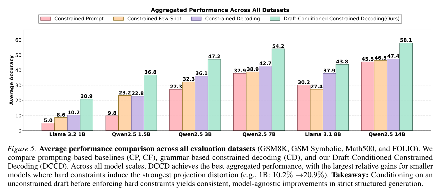
Paper's Figure 5 (caption: "Average performance comparison across all evaluation datasets... DCCD achieves the best aggregated performance, with the largest relative gains for smaller models... 1B: 10.2%→20.9%").
DCCD (green) is highest at every scale vs Constrained Prompt (CP), Constrained Few-Shot (CF), and grammar CD. Reading the bars: Qwen2.5-1.5B jumps 22.8→36.8, 7B 42.7→54.2, 14B 47.4→58.1. The clearest signal supporting the theory is the shape: the smaller the model (lower feasible mass, worst projection tax), the larger the DCCD lift — exactly what §4's mechanism predicts. (Note the Llama-3.2-1B green bar reads 20.9 here, matching the caption's "→20.9%"; an L1-extracted table had a transcription ambiguity, resolved in favor of the figure.)
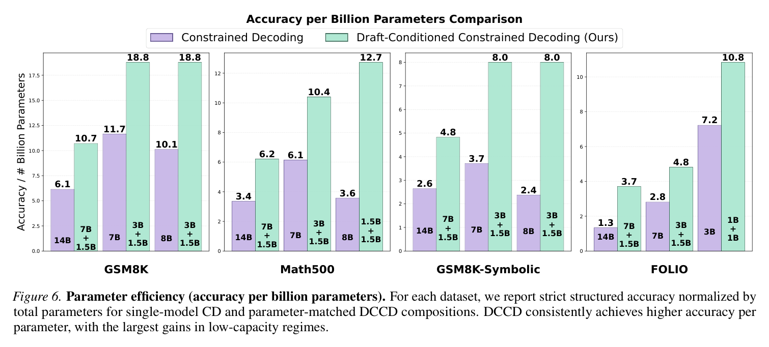
Paper's Figure 6 (caption: "Parameter efficiency (accuracy per billion parameters)... DCCD consistently achieves higher accuracy per parameter, with the largest gains in low-capacity regimes").
Each cluster compares a single-model CD (purple, e.g. 14B) against a parameter-matched DCCD composition (green, e.g. 7B+1.5B). DCCD accuracy-per-B roughly triples on GSM8K (6.1→18.8) and MATH500 (3.4→12.7). This is the load-bearing efficiency claim: splitting a fixed parameter budget into drafter+projector beats spending it all on one constrained model.
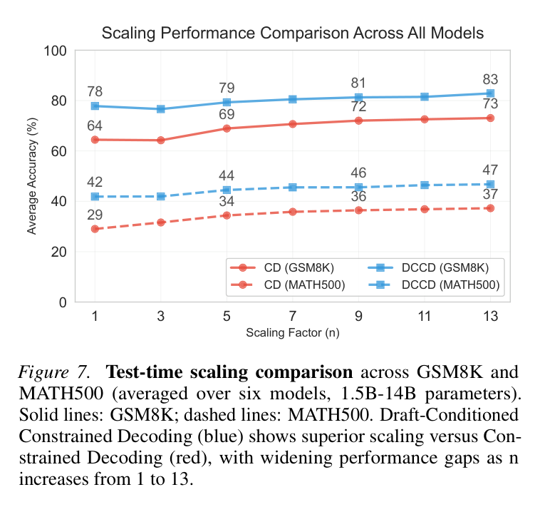
Paper's Figure 7 (caption: "Test-time scaling comparison across GSM8K and MATH500... DCCD (blue) shows superior scaling versus Constrained Decoding (red), with widening performance gaps as n increases from 1 to 13").
Best-of-$K$ draft selection lets DCCD absorb test-time compute more productively than repeated constrained sampling: on GSM8K DCCD 78→83 vs CD 64→73; on MATH500 42→47 vs 29→37. Gains saturate around $n\approx7$ (best drafts already sampled), and the gap never closes — allocating compute to diverse drafts beats resampling under the constraint.
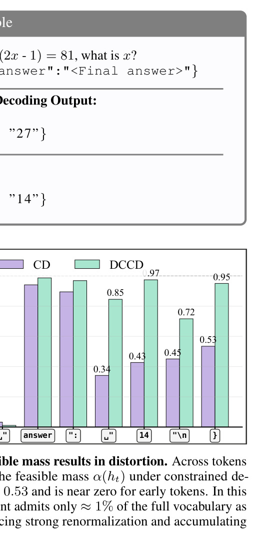
Paper's Figure 3 (feasible-mass toy example: for the answer to $3(2x-1)=81$, CD emits valid-but-wrong "27", DCCD emits correct "14"; per-token $\alpha$ bars).
This is the empirical anchor for the projection-tax story: on the forced formatting/answer tokens CD's feasible mass is often ≤0.53 and near-zero for early tokens (~1% of vocab feasible), while DCCD lifts each to 0.85–0.97. Low $\alpha$ at many steps is precisely what accumulates into distortion and the valid-but-wrong "27".
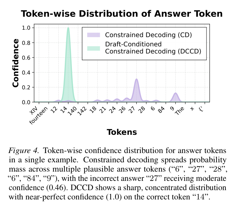
Paper's Figure 4 (caption: "Constrained decoding spreads probability mass across multiple plausible answer tokens... incorrect answer '27' receiving moderate confidence (0.46). DCCD shows a sharp, concentrated distribution with near-perfect confidence (1.0) on the correct token '14'").
Where CD smears mass across 27/28/6/84/9, DCCD collapses onto the correct 14. The reasoning content was already in the draft; conditioning makes the answer slot near-deterministic once the schema is satisfied.
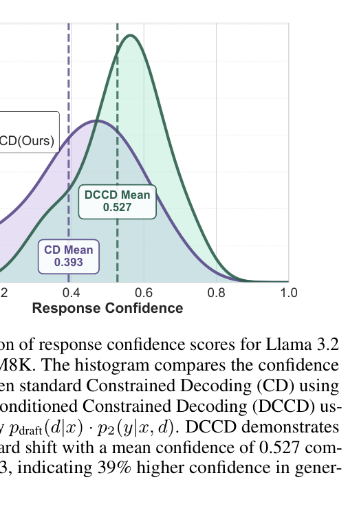
Paper's Figure 7 in source text / response-confidence histogram (Llama-3.2-3B, GSM8K): DCCD mean 0.527 vs CD 0.393, a +39% rightward shift.
Notably DCCD's confidence is the joint $p_{\mathrm{draft}}(d\mid x)\cdot p_2(y\mid x,d)$ — a product of two stages — yet still exceeds single-stage CD. Separating reasoning from formatting raises confidence even though naively multiplying two probabilities should lower it.
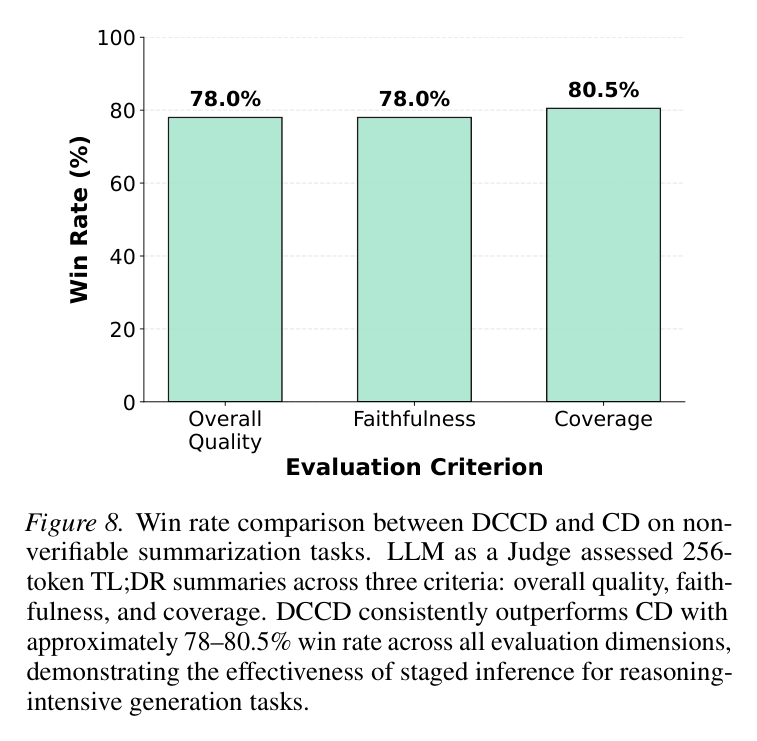
Paper's Figure 8 (caption: "Win rate comparison between DCCD and CD on non-verifiable summarization tasks... approximately 78–80.5% win rate across all evaluation dimensions").
LLM-as-judge on 256-token TL;DR summaries: DCCD wins ~78% (quality), 78% (faithfulness), 80.5% (coverage), showing the staged recipe generalizes beyond verifiable math to open-ended generation.
6. 论证链 #
| # | Step | Paper-internal support |
|---|---|---|
| 1 | CD masks+renormalizes ⇒ per-step reverse-KL distortion $=\log\frac1{\alpha(h_t)}$ | Eq.4–5 derivation |
| 2 | Distortions add over the trajectory ⇒ cumulative "projection tax" $\sum_t\log\frac1{\alpha}$; reweights even valid strings by $\prod_t\alpha^{-1}$, biasing toward easy-to-project (locally valid) prefixes | Eq.7–8, toy example, Fig.3 |
| 3 | Feasible mass $\alpha$ depends on conditioning context, which is free at inference ⇒ appending a draft $d$ gives $\alpha(h_t;d)\gg\alpha(h_t)$ | Eq.10–11 |
| 4 | Instantiate $d$ as an unconstrained draft $y$; constrain conditioned on $(x,y)$ ⇒ same exact validity ($A(h_t)$ unchanged), smaller distortion | Eq.12–15, Alg.1 |
| 5 | Smaller distortion (KL) ⇒ tighter worst-case utility-loss bound via Pinsker on validity-gated utility | Eq.16–18 (Appendix A) |
| 6 | Best-of-$K$ by cumulative $\log\alpha$ picks the least-distorted trajectory ⇒ test-time compute converts to accuracy | Alg.1 selector, Fig.7 |
| 7 | Empirically: best strict accuracy at all 1B–14B scales, largest lift for small models, better param-efficiency and scaling | Fig.1, Fig.5, Fig.6, Fig.7 |
7. 实现 cross-reference #
关键实现细节 (easy-to-miss tricks).
核心技术壁垒 (deep-dive). The single hardest-to-replicate insight is not the two-step procedure (obvious in hindsight) but the reframing: proving that the quality-validity tradeoff is a KL-projection artifact whose magnitude is $\log\frac1{\alpha(h_t)}$, then observing $\alpha$ is a free variable at inference because it depends on conditioning context (Eq.10). This turns "constraints hurt accuracy" from an accepted cost into a reducible distortion, and it is what justifies keeping the constraint set fully intact (no relaxation, exact guarantees) while recovering unconstrained-level accuracy. Everything else (best-of-$K$, param-efficient drafter/projector split) follows mechanically from this identity.
Implementation stack. CD baseline uses XGrammar integrated with vLLM; JSON tasks via Pydantic schemas (class MATHSchema(BaseModel): steps: List[str]; answer: str), symbolic/logical tasks via Lark-style CFGs (GSM-Symbolic < grammar; FOLIO first-order-logic grammar verified by Prover9). DCCD's own decoding code is [实现未公开] — no repository link in the source; the method is described only as pseudocode (Algorithm 1) plus the XGrammar/vLLM masking backend.
8. Serving deployment considerations #
9. Training recipe & LLM-specific asks #
This is an inference-time method, not a model release — several deep-model rows are therefore N/A:
| Stage | Goal | Data (tokens + mix) | LR schedule | Context | Techniques |
|---|---|---|---|---|---|
| (any) | — | — | — | — | N/A — DCCD is training-free; no pre-training, mid-training, SFT, or post-training is performed. Uses off-the-shelf Llama-3.x / Qwen2.5 Instruct checkpoints. |
10. Open questions (LLM-specific angles) #
Appendix: 模型架构图 #
N/A — this paper is an inference-time decoding procedure, not a model release. There is no released model architecture, no official modeling_*.py, and no config.json to reverse-engineer (Table 1 uses stock Llama-3.x / Qwen2.5 checkpoints whose architectures are documented elsewhere). The only "architecture" is the two-stage decoding control flow, drawn as a Mermaid sequence in §3. No per-block attention/FFN diagrams apply because the method leaves the underlying transformer untouched.