Attention Residuals
Attention Residuals — L2 #
Kimi Team: Guangyu Chen, Yu Zhang, Jianlin Su, Weixin Xu et al. (37 authors, Moonshot AI) 2026-03 | https://arxiv.org/abs/2603.15031
§1 TL;DR #
AttnRes 用 depth-wise softmax attention(每层一个伪 query $\mathbf{w}_l$)替代固定权重 1 的残差累加,解决 PreNorm dilution;Block AttnRes 将层分 N 块把内存从 $O(Ld)$ 降至 $O(Nd)$。1.25× compute equivalence,Kimi Linear 48B 全面提升(GPQA +7.5),训练开销 <4%。
§2 痛点 · 方法 · 结果 #
Q1 痛点 #
标准 PreNorm Transformer 的残差更新为 $\mathbf{h}_l = \mathbf{h}_{l-1} + f_l(\mathbf{h}_{l-1})$,每层输出以固定权重 1 累加。展开后 $\mathbf{h}_L = \sum_{i=0}^{L-1} \mathbf{v}_i$,每个 $\mathbf{v}_i$ 因 PreNorm 约束有 $\|\mathbf{v}_i\| \approx O(1)$,但累积态 $\|\mathbf{h}_l\| \approx O(l)$,导致三个问题:
- PreNorm dilution:第 $i$ 层输出在第 $l$ 层的相对贡献衰减为 $\sim 1/l$,深层被迫学更大输出以保持影响力
- 无选择性访问:所有先前层以同一权重混合,attention 子层和 MLP 子层共享同一聚合态
- 不可逆信息丢失:早期层信息一旦被稀释,后续层无法恢复
- 收敛性:AttnRes 引入 softmax 非线性到 forward pass 中,是否影响训练收敛的理论保证?零初始化让起始等价于均匀平均(标准残差的一个变体),但从均匀→学习后权重的过渡没有形式化分析
- Block vs Full 近似误差 bound:$N$ 个 block 对 $L$ 个 layer 的近似质量应可用信息论/矩阵近似理论量化
- Gradient flow 分析:论文观察到更均匀的梯度分布(Fig 5),但未给出 AttnRes 下梯度传播的形式化表达
block_attn_res()— 核心 inter-block attention(README),对应论文公式 3.1–3.2forward()— 单层 forward pass 含两次 AttnRes 注入(README),展示 block boundary logic- Two-phase online softmax merge:Phase 1 对已完成 block 做 batch attention query(pseudo-query 是参数不依赖输入,可预计算);Phase 2 在 intra-block forward 过程中用 online softmax 将 partial block 与 pre-computed 结果合并。公式为:
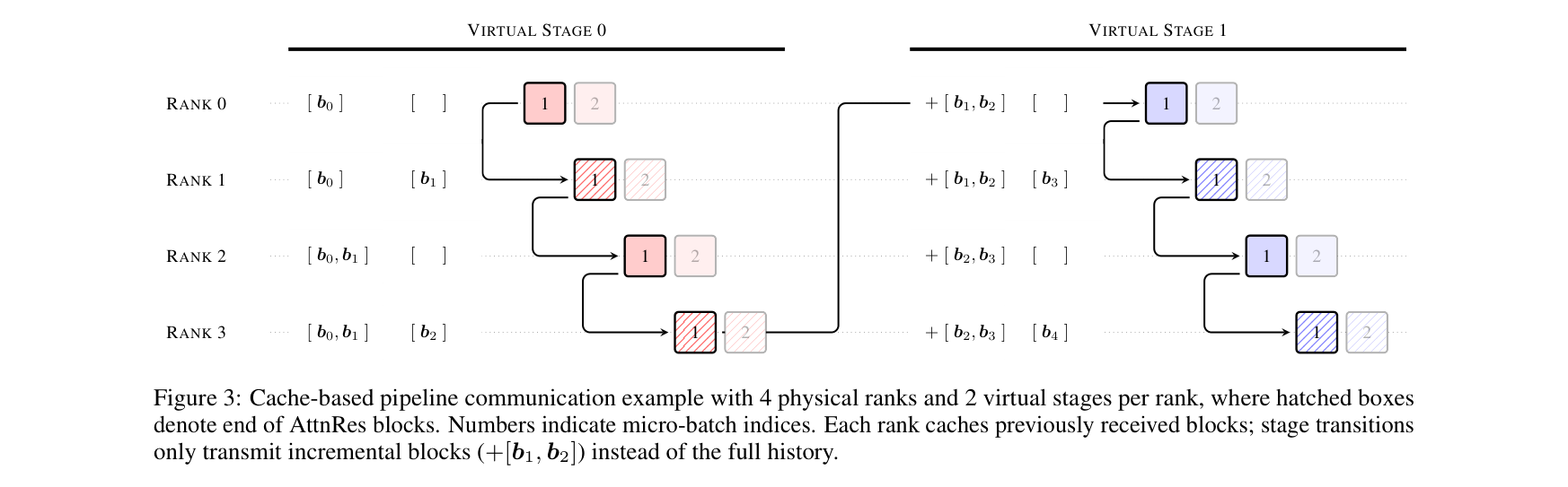
- Cross-stage caching for pipeline parallelism:Interleaved pipeline schedule 下,block reps 在 virtual stages 间本地缓存,避免每个 micro-batch chunk 都重传。Per-transition 通信从 $O(C)$ 降到 $O(P)$。
- Sequence-sharded prefill:长上下文下 block reps 按 TP 分片,每 device 只存 $O(N \cdot T/P_{\text{tp}} \cdot d)$。128K context 从 15GB 压到 <0.3GB。
- Pseudo-query 零初始化:$\mathbf{w}_l = \mathbf{0}$ 使所有 logits 在初始化时相等,softmax 输出均匀分布 $\alpha_{i \to l} = 1/l$。这保证 AttnRes 在训练开始时退化为标准残差的均匀平均版本,是训练稳定性的关键。非零初始化在消融中显著 underperform。
- RMSNorm 加在 key 而非 value 上:消融显示去掉 RMSNorm 导致 loss 从 1.737 升到 1.750。原因:不同 block 的 summary $\mathbf{b}_n$ 因包含不同数量层的累加而范数差异大,RMSNorm 确保 attention 基于内容而非范数竞争。
- 训练代码:未公开完整实现。最接近的开源参考为 Hyper-Connections (mHC) 的实现(用于对比 baseline)
- 社区复现:截至 2026-05 未发现独立复现报告
- 生产采用:Kimi Linear (48B-A3B) 和 K2.5 已部署 Block AttnRes。其他已知采用者:无公开报告
- AttnRes 与 input-dependent query 的后续:论文消融显示 input-dependent query (loss 1.731) 优于 pseudo-query (1.737),但因推理 sequential 依赖而弃用——这是一个明确的 future work 方向
问题定义:给定 $L$ 层 Transformer,输入 token embedding $\mathbf{h}_0$,每层变换 $f_l$,设计深度聚合机制使各层贡献不因累积而被稀释。标准损失函数为 language modeling cross-entropy,AttnRes 不改变损失,只改变 forward pass 中的深度聚合方式。
Q2 方法 #
Full AttnRes 将固定累加替换为 depth-wise softmax attention:
$$\mathbf{h}_l = \sum_{i=0}^{l-1} \alpha_{i \to l} \cdot \mathbf{v}_i$$
$$\alpha_{i \to l} = \frac{\exp(\mathbf{w}_l^\top \operatorname{RMSNorm}(\mathbf{k}_i))}{\sum_{j=0}^{l-1} \exp(\mathbf{w}_l^\top \operatorname{RMSNorm}(\mathbf{k}_j))}$$
其中 $\mathbf{w}_l \in \mathbb{R}^d$ 为每层学习的伪 query(零初始化),$\mathbf{k}_i = \mathbf{v}_i$ 为第 $i$ 层输出。每层增加的参数仅为一个 $d$ 维向量和一个 RMSNorm——对 $d=4096$, $L=64$ 的模型约 524K 参数(~0.005%)。
核心 insight 是 深度-序列对偶 (depth-sequence duality):标准残差 = 沿深度的 RNN(固定单元权重),就像 Transformer 用 attention 替代了时间维 RNN,AttnRes 用 attention 替代了深度维 RNN。
Block AttnRes 将 $L$ 层分成 $N$ 个 block,block 内标准残差,block 间做 softmax attention over block summaries $\mathbf{b}_n = \sum_{i \in \text{block}_n} \mathbf{v}_i$,内存从 $O(Ld)$ 降至 $O(Nd)$。
| Before(Standard Residual) | After(AttnRes) | |
|---|---|---|
| 聚合公式 | $\mathbf{h}_l = \mathbf{h}_{l-1} + f_l(\mathbf{h}_{l-1})$ | $\mathbf{h}_l = \sum_i \alpha_{i \to l} \cdot \mathbf{v}_i$ |
| 权重类型 | 固定 (all ones) | Learned, softmax-normalized |
| Input-dependent | No | Yes(via pseudo-query) |
| M 矩阵结构 | All-ones lower-triangular | Dense, rank-$l$, input-dependent |
| 范数增长 | $O(L)$ monotonic | Bounded periodic |
核心技术壁垒:不在 Full AttnRes 的公式(简洁直接),而在 Block AttnRes 的系统工程——(1) 两阶段在线 softmax 合并(已完成 block 的 pre-computed attention + in-progress partial block 的 online merge),(2) pipeline parallelism 下跨 stage 的 block representation 缓存通信协议(将 per-transition 通信从 $O(C)$ 降到 $O(P)$),(3) 序列分片 prefill(128K context 从 15GB 压到 <0.3GB)。三者联合实现 <4% 训练开销和 <2% 推理延迟,是将理论方法变为 production-ready 的关键壁垒。
Q3 结果 #
Scaling law(194M–528M,5 个模型尺度):Block AttnRes 在相同 loss 下节省 ~1.25× compute。拟合幂律 $\mathcal{L} = a \times C^{-b}$:
| Variant | $a$ | $b$ | Loss @ max compute |
|---|---|---|---|
| Baseline | 1.891 | 0.057 | 1.719 |
| Block AttnRes | 1.870 | 0.058 | 1.693 |
| Full AttnRes | 1.865 | 0.057 | 1.692 |
Kimi Linear 48B (3B activated MoE),1.4T tokens pre-training:
| Benchmark | Baseline | AttnRes | Delta |
|---|---|---|---|
| GPQA-Diamond | 36.9 | 44.4 | +7.5 |
| Math | 53.5 | 57.1 | +3.6 |
| HumanEval | 59.1 | 62.2 | +3.1 |
| MMLU | 73.5 | 74.6 | +1.1 |
| C-Eval | 79.6 | 82.5 | +2.9 |
所有 15 个 benchmark 均持平或改善。多步推理任务(GPQA, Math, HumanEval)收益最大,符合深度选择性改善组合推理的假设。
§3 架构 / 方法图 #
AttnRes 架构总览 #
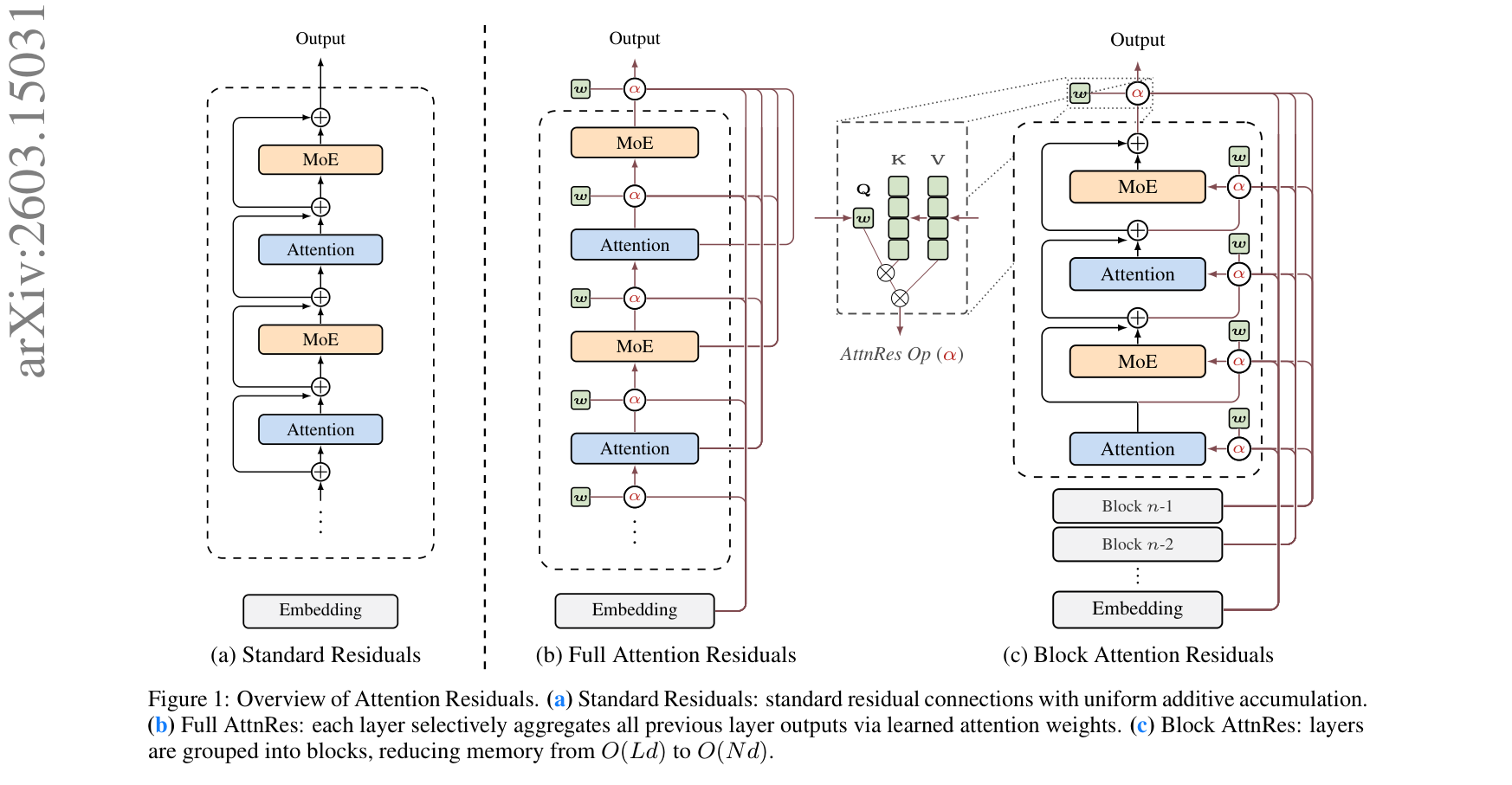
Paper's Figure 1, verbatim (caption: "Overview of Attention Residuals. (a) Standard Residuals: standard residual connections with uniform additive accumulation. (b) Full AttnRes: each layer selectively aggregates all previous layer outputs via learned attention weights. (c) Block AttnRes: layers are grouped into blocks, reducing memory from O(Ld) to O(Nd).").
三列对比一目了然:(a) 标准残差逐层累加(每条边权重=1),(b) Full AttnRes 每层对所有先前层做 softmax attention(边权重 $\alpha_{i \to l}$ 可变),(c) Block AttnRes 将层分组、block 内标准累加、block 间做 attention。关键视觉线索:(b) 的连接密度远高于 (a),但 (c) 通过 block 压缩把密度降回可控范围。
Depth mixing matrix 统一视角 #

Paper's Figure 9, verbatim (caption: depth-mixing matrices M for Standard residuals, Highway, mHC, DenseFormer, Full AttnRes, Block AttnRes).
论文 §6.2 将所有残差变体统一到 depth mixing matrix $M \in \mathbb{R}^{L \times L}$ 框架下:$\mathbf{h}_l = \sum_{i=0}^{l-1} M_{i \to l} \cdot \mathbf{v}_i$。标准残差的 $M$ 是 all-ones 下三角(rank-1, input-independent),Highway 是 1-semiseparable with scalar gates,mHC 是 $m$-semiseparable,DenseFormer 有 learned but input-independent 标量——所有这些都对应 depth-wise linear attention。AttnRes 是首个使用 depth-wise softmax attention 的方法,$M$ dense 且 input-dependent。这与序列维度上 RNN→Transformer 的转变完全平行。
Block AttnRes 伪代码 #
def block_attn_res(blocks: list[Tensor], partial_block: Tensor,
                   proj: Linear, norm: RMSNorm) -> Tensor:
    V = torch.stack(blocks + [partial_block])  # [N+1, B, T, D]
    K = norm(V)                                 # RMSNorm on keys
    logits = torch.einsum('d, n b t d -> n b t',
                          proj.weight.squeeze(), K)
    h = torch.einsum('n b t, n b t d -> b t d',
                     logits.softmax(0), V)
    return h
每个 Transformer 层执行两次 block_attn_res(attn 子层前 + MLP 子层前),各有独立的 proj 和 norm。Block 边界由 layer_number % (block_size // 2) == 0 决定。
系统优化(§4) #
| 优化 | 机制 | 效果 |
|---|---|---|
| Cross-stage caching | Block reps 缓存在本地,跨 pipeline stage 复用 | 通信从 $O(C)$ 降到 $O(P)$ |
| Two-phase inference | Phase 1: batch pre-compute inter-block attention; Phase 2: online softmax merge with partial block | <2% latency overhead |
| Sequence-sharded prefill | Block reps 按 TP 分片 | 128K context: 15GB → <0.3GB |
§4 作者证明 #
无形式化作者证明 — 仅实证
论文无收敛定理、无 variance bound、无 loss decomposition 证明。核心理论贡献是 §6.2 的 structured-matrix taxonomy(描述性框架而非形式化定理)。以下为符号表和方程物理意义分析。
符号表 #
| Symbol | Definition | Physical meaning |
|---|---|---|
| $\mathbf{h}_l$ | Hidden state at layer $l$ | 第 $l$ 层的输入表示 |
| $\mathbf{v}_i$ | Output of layer $i$: $f_i(\mathbf{h}_i)$ | 第 $i$ 层变换后的增量 |
| $\mathbf{w}_l$ | Learned pseudo-query $\in \mathbb{R}^d$ | 第 $l$ 层的深度偏好向量(零初始化) |
| $\alpha_{i \to l}$ | Softmax attention weight | 第 $i$ 层对第 $l$ 层的贡献权重 |
| $\mathbf{b}_n$ | Block summary: $\sum_{i \in \text{block}_n} \mathbf{v}_i$ | 第 $n$ 个 block 内所有层输出之和 |
| $M_{i \to l}$ | Depth mixing matrix element | 统一框架下第 $i$ 层对第 $l$ 层的权重 |
| $\mathcal{L}$ | Validation loss | 语言建模 cross-entropy |
| $C$ | Compute (PFLOP/s-days) | 训练计算量 |
| $a, b$ | Scaling law coefficients | $\mathcal{L} = a \times C^{-b}$ |
方程物理意义 #
标准残差展开:
$$\mathbf{h}_L = \sum_{i=0}^{L-1} \mathbf{v}_i$$
所有层输出以 unit weight 求和。$M$ 矩阵为 all-ones 下三角。因 PreNorm 保证 $\|\mathbf{v}_i\| \approx O(1)$,$\|\mathbf{h}_L\| \approx O(L)$——dilution 的数学根源。
AttnRes 聚合:
$$\mathbf{h}_l = \sum_{i=0}^{l-1} \alpha_{i \to l} \cdot \mathbf{v}_i, \quad \sum_i \alpha_{i \to l} = 1$$
Softmax 归一化使 $\|\mathbf{h}_l\|$ 不再随 $l$ 无界增长(bounded by max $\|\mathbf{v}_i\|$)。竞争机制使高相关源层被放大、低相关源层被抑制。
Block summary:
$$\mathbf{b}_n = \sum_{i \in \text{block}_n} \mathbf{v}_i$$
Block 内仍用标准累加(保持局部信息流),block 间做 softmax attention。$N$ 个 block + embedding 构成 $N+1$ 个候选,attention 复杂度从 $O(L)$ 降到 $O(N)$。
Scaling law fit:
$$\mathcal{L}_{\text{baseline}} = 1.891 \times C^{-0.057}, \quad \mathcal{L}_{\text{block}} = 1.870 \times C^{-0.058}$$
Exponent 基本一致($\approx 0.057$–$0.058$),improvement 体现为 multiplicative offset——AttnRes 是 constant-factor improvement 而非改变 scaling 行为。
应有但论文未提供的保证 #
6 项验证 #
| # | Check | Result |
|---|---|---|
| 1 | 量纲一致性: $\alpha_{i \to l}$ 无量纲概率,$\sum_i \alpha_{i \to l} = 1$ | ✓ softmax 输出 $\in (0,1)$, sum = 1 |
| 2 | 退化路径: $\mathbf{w}_l = \mathbf{0} \Rightarrow$ 所有 logits 相等 $\Rightarrow \alpha_{i \to l} = 1/l$ (均匀平均) | ✓ 开始时退化为均匀聚合 |
| 3 | 边界条件: $l=1 \Rightarrow \mathbf{h}_1 = \alpha_{0 \to 1} \cdot \mathbf{v}_0 = \mathbf{v}_0$ (只有 embedding) | ✓ 单源 softmax 退化为 identity |
| 4 | Scaling 一致性: exponent $b \approx 0.057$–$0.058$ 跨三种 variant 一致 | ✓ 改变 offset 不改变 scaling 行为 |
| 5 | Block 近似收敛: Block size $S=1$ (= Full) → $S=2,4,8$ → $S=16,32$ 单调退化 | ✓ Table/Fig 3 验证 |
| 6 | 参数效率: 每层增加 $2d$ 参数 (query + RMSNorm gain),总增量 $2Ld \ll d^2 L$ | ✓ 对 $d=4096$, $L=64$: 524K vs ~10B |
§5 实验与数据 #
Scaling Law(194M–528M) #
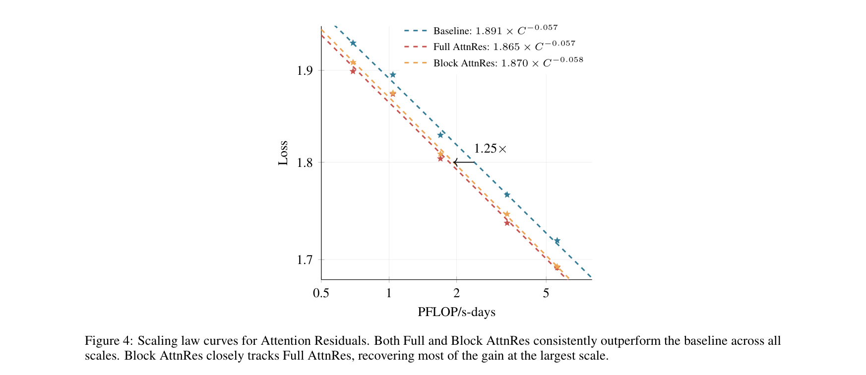
Paper's Figure 4, verbatim (caption: Scaling curves showing fitted power laws for Baseline, Block AttnRes, and Full AttnRes).
三条曲线斜率一致但 offset 不同:Full AttnRes < Block AttnRes < Baseline 在所有 compute level。在 matched loss 下 Block AttnRes 节省 ~1.25× compute——等价于"免费"多训 25%。Full 与 Block 的差距随规模收窄:最大 config(528M)仅 0.001。
| # Act. Params | Tokens | Baseline | Block AttnRes | Full AttnRes | mHC(-lite) |
|---|---|---|---|---|---|
| 194M | 38.7B | 1.931 | 1.909 | 1.899 | 1.906 |
| 241M | 45.4B | 1.895 | 1.875 | 1.874 | 1.869 |
| 296M | 62.1B | 1.829 | 1.809 | 1.804 | 1.807 |
| 436M | 87.9B | 1.766 | 1.746 | 1.737 | 1.747 |
| 528M | 119.0B | 1.719 | 1.693 | 1.692 | 1.694 |
mHC(-lite) 在 241M 规模略优(1.869 vs 1.874/1.875),但在所有其他规模上 Full AttnRes 胜出。
Training Dynamics #
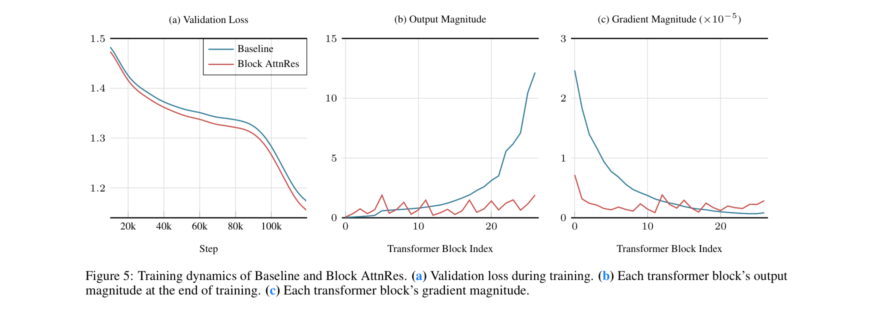
Paper's Figure 5, verbatim (caption: Training dynamics comparison showing output magnitudes and gradient norms across depth for Baseline vs Block AttnRes).
左图(output magnitudes):Baseline 单调增长($O(L)$ PreNorm dilution 的直接证据),AttnRes 呈 bounded periodic pattern——block 边界处 softmax 归一化重置累积,范数周期性回落。右图(gradient norms):Baseline 早期层梯度不成比例地大(identity path 放大敏感度),AttnRes 梯度分布更均匀。这两个观察是 AttnRes "为什么能 work" 的核心训练动态证据:softmax 归一化同时解决了前向的范数爆炸和反向的梯度不均匀。
Architecture Sweep #
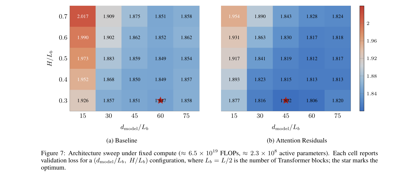
Paper's Figure 7, verbatim (caption: Architecture sweep under fixed compute: validation loss vs. d_model/L_b ratio for Baseline and AttnRes).
固定 compute $\approx 6.5 \times 10^{19}$ FLOPs 下,Baseline 最优 width/depth 比 $d_{\text{model}}/L_b \approx 60$(偏宽浅),AttnRes 最优比 $\approx 45$(偏窄深)。AttnRes 在所有 configuration 上均优于 Baseline,但在更深/更窄配置上优势更大——标准残差是 depth utility 的瓶颈,AttnRes 解锁了深度的价值。
Depth-wise Attention Patterns #
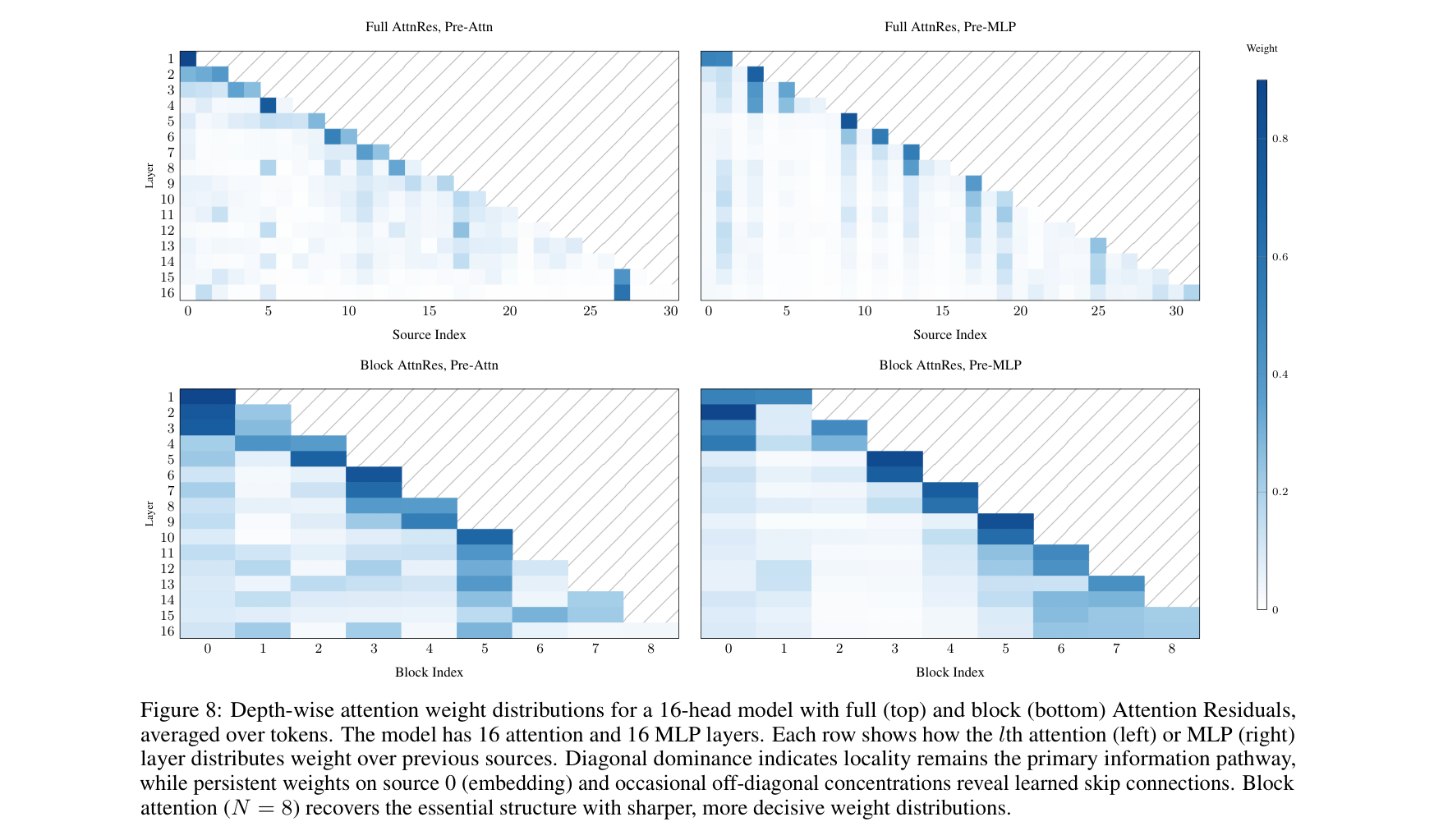
Paper's Figure 8, verbatim (caption: Depth-wise attention weight distributions showing which layers attend to which).
可视化 $\alpha_{i \to l}$ 矩阵揭示三个 striking patterns:(1) Locality preserved——对角线主导,每层仍最关注其前驱;(2) Embedding persistence——layer 0 (token embedding) 在整个深度上保持显著权重,模型学会了持续参考原始输入;(3) Attention vs MLP 分化——pre-attention 层有更宽的 receptive field(跨更远的层取信息),pre-MLP 层更依赖 recent information。
Ablation Study(436M, 16 层) #
| Variant | Val loss |
|---|---|
| Baseline (PreNorm) | 1.766 |
| DenseFormer (fixed scalars) | 1.767 |
| mHC | 1.747 |
| Full AttnRes | 1.737 |
| Block AttnRes ($N=8$) | 1.746 |
| w/ sigmoid (not softmax) | 1.741 |
| w/ input-dependent query | 1.731 |
| w/ multi-head depth attn | 1.752 |
| w/o RMSNorm | 1.750 |
关键发现:(1) DenseFormer 无效(1.767 ≈ baseline 1.766)——input-independence 是瓶颈,不是 cross-layer access 的缺失;(2) softmax > sigmoid(1.737 vs 1.741)——竞争性归一化创造更锐利的选择;(3) multi-head depth attention 反而伤害(1.752)——层输出要么整体相关、要么整体不相关,per-channel 路由无益;(4) RMSNorm 关键(1.737 vs 1.750 without)——不加则大范数层主导 attention;(5) input-dependent query 最优(1.731)但不实用——需 $d \times d$ 矩阵且强制 sequential inference。
Kimi Linear 48B Pre-training #
| 维度 | 数值 |
|---|---|
| Total / Active params | 48B / 3B (MoE) |
| Layers | 27 transformer (54 sublayers) |
| Block size | 6 sublayers (3 transformer layers) |
| Pre-train tokens | 1.4T |
| Optimizer | Muon + WSD |
| Context | 4K → 32K |
| AttnRes injections / layer | 2 (attn-pre + mlp-pre) |
| Training overhead | <4% |
| Inference latency overhead | <2% |
| GPU hours | [论文未披露] |
| MFU | [论文未披露] |
所有 15 个 benchmark 持平或提升(Table 3),compositional reasoning 类任务收益最大(GPQA +7.5, Math +3.6, HumanEval +3.1),knowledge-oriented 任务收益较小(MMLU +1.1)。
Block Size Sensitivity #
Paper's Figure 3, verbatim (caption: Block size ablation: validation loss as a function of block size S).
Block size $S = 2, 4, 8$ 的 loss 差距在 0.004–0.006 以内(接近 Full AttnRes),$S = 16, 32$ 逐步退化到 baseline 附近。$N \approx 8$ blocks 是实践甜点:深度信息结构是 remarkably coarse-grained 的——8 个 summary 就捕获了几乎全部 depth-wise selectivity 的价值。
Dataset Analysis #
[论文未披露训练数据组成] — 使用 Kimi Linear 的预训练数据(web/code/math/chat 比例、质量过滤、contamination check 均未公开)。
§6 论证链 #
| Step | Premise | Conclusion | Evidence | ||||
|---|---|---|---|---|---|---|---|
| 1 | PreNorm 下 $\ | \mathbf{v}_i\ | \approx O(1)$ 但 $\ | \mathbf{h}_l\ | \approx O(l)$,第 $i$ 层贡献相对衰减为 $\sim 1/l$ | 标准残差存在 PreNorm dilution:深层被迫学更大输出,层间信息流缺乏选择性 | §2 形式推导 + Fig 5 左图(output magnitudes 单调增长) |
| 2 | 序列维度上 RNN→Transformer(attention 替代 recurrence)大幅提升表达力;残差是深度维度的 "RNN"(固定权重累加 = linear attention with all-ones M) | 用 depth-wise softmax attention 替代 fixed accumulation 应带来类似收益(depth-sequence duality) | §6.2 structured-matrix framework: 标准残差 = depth-wise linear attention, AttnRes = depth-wise softmax attention | ||||
| 3 | Full AttnRes 每层对所有 $l$ 个先前层做 softmax attention,单层增加 $\sim 2d$ 参数;Block AttnRes 将 $L$ 层分 $N$ block 降低到 $O(N)$ 候选 | 在可控开销下实现 input-dependent depth-wise selection | Table 4 ablation(Full: 1.737, Block: 1.746, Baseline: 1.766)+ §4 系统优化(<4% training, <2% inference) | ||||
| 4 | 5 个模型尺度的 scaling 实验:AttnRes 曲线在所有 compute 水平一致低于 baseline;exponent 不变,改善为 constant offset | AttnRes 是 fundamental 而非 scale-dependent 的改进;Block AttnRes ≈ 1.25× compute equivalence | Fig 4 scaling curves + 拟合系数 $a=1.870$ vs $1.891$, $b=0.058$ vs $0.057$ | ||||
| 5 | Kimi Linear 48B (3B activated) 1.4T tokens pre-training:15 benchmarks 全面持平或提升,GPQA +7.5, Math +3.6 | AttnRes 在生产规模 MoE 模型上有效,compositional reasoning 受益最大 | Table 3 全 benchmark 比较 | ||||
| 6 | 可视化 $\alpha_{i \to l}$:对角线主导(locality),embedding 持续高权重,attention 子层 broader receptive field | 模型自主学出了有意义的 depth routing pattern——不是随机分配而是有结构的信息流优化 | Fig 8 attention pattern 可视化 |
§7 实现 cross-reference #
代码引用 #
官方仓库 MoonshotAI/Attention-Residuals 提供 PyTorch 伪代码:
完整训练代码和 pipeline parallelism 的 cross-stage caching 实现 [实现未公开]——仓库仅有 README 级伪代码,无可运行的训练/推理代码。生产部署在 Kimi Linear(arXiv 2510.26692)中。
核心技术壁垒展开 #
Block AttnRes 的 <4% training overhead 依赖三个系统组件的精确协同:
$$h_l = \frac{e^{m_1 - m} \cdot o_1 + e^{m_2 - m} \cdot o_2}{e^{m_1 - m} \cdot \ell_1 + e^{m_2 - m} \cdot \ell_2}$$
其中 $m = \max(m_1, m_2)$。这是 Flash Attention 的 online softmax 技巧在深度维度上的应用。