Chimera: Latency- and Performance-Aware Multi-agent Serving for Heterogeneous LLMs
Chimera: Latency- and Performance-Aware Multi-agent Serving for Heterogeneous LLMs — L2 #
1. TL;DR #
Middleware atop vLLM that serves multi-agent workflows on a mix of LLM sizes/families. It couples a semantic router (per-model success confidence), a CPU QRF that predicts a workflow's total remaining output tokens, and an in-flight-token load monitor to pick the strongest model within a latency slack and schedule by Shortest-Total-Job-First. Traces the best latency–performance Pareto frontier: 1.2–2.4× lower latency, +8–9.5 pp performance, ≤2.2% overhead.
2. Q1 / Q2 / Q3 #
Q1 — 痛点. Multi-agent tasks run as multi-stage workflows (a query fans out into dependent LLM calls, each consuming prior stages' output). Two facts break existing serving: (a) prior serving systems assume a homogeneous cluster (identical replicas), so they never decide which model of differing capacity should serve requests of differing difficulty; (b) prior routers treat latency as a static per-model attribute, ignoring that routing a hard request to a slow, capable model amplifies queue congestion and hurts other workflows. The result is an intrinsic latency–performance trade-off that neither camp addresses jointly.
Q2 — 方法. Chimera is a predictive scheduler middleware sitting between agent apps and a pool of heterogeneous inference engines. Per request it computes: (i) Semantic Router — ModernBERT-large multi-label head emitting an independent sigmoid confidence $q[m]$ per candidate model; (ii) Length Predictor — a Quantile Random Forest predicting the workflow-total remaining output tokens $\hat{y}$ (used as scheduling priority); (iii) Activity Monitor — per-engine map of in-flight predicted tokens; (iv) Load Balancer — estimates each model's time-to-last-token from in-flight tokens, then picks the highest-confidence model that stays within $(1+\tau)$ of the fastest model's latency and beats current confidence by margin $\Delta s$. Requests are queued by Shortest-Total-Job-First on $\hat{y}$, with aging-based anti-starvation.
核心技术壁垒: the workflow-level total-remaining-output-length signal $Y_r=\sum_{j=i}^{N_p}\text{OutTokens}(p,j)$ — predicting not just this stage's output but the sum over all future stages of a multi-agent program, cheaply on CPU and robustly under heavy tails, then feeding it simultaneously as (a) scheduling priority and (b) the load estimate that drives model routing. This coupling is what turns two independently-studied signals (routing, length prediction) into a joint latency+performance win.
Q3 — 结果. Across APPS (code) and MATH (math) on RTX A6000 clusters mixing 1.5B–14B Qwen/Llama/Ministral models, Chimera dominates vLLM, MLFQ, and LTR on the $(C,S)$ frontier: e.g. APPS Qwen1.5+7B = 3.4× speedup and +16.0 pp over vLLM; near the vLLM(STJF) oracle on the hard long-output config. Scheduler overhead ≤2.2% of E2E latency. Gains are large on APPS (8.2–19.6 pp) but small on MATH (1.2–5.0 pp).
3. 架构 / 方法图 #
Chimera is a middleware layer, not a new engine — it wraps stock vLLM engines and only makes the dispatch decision.
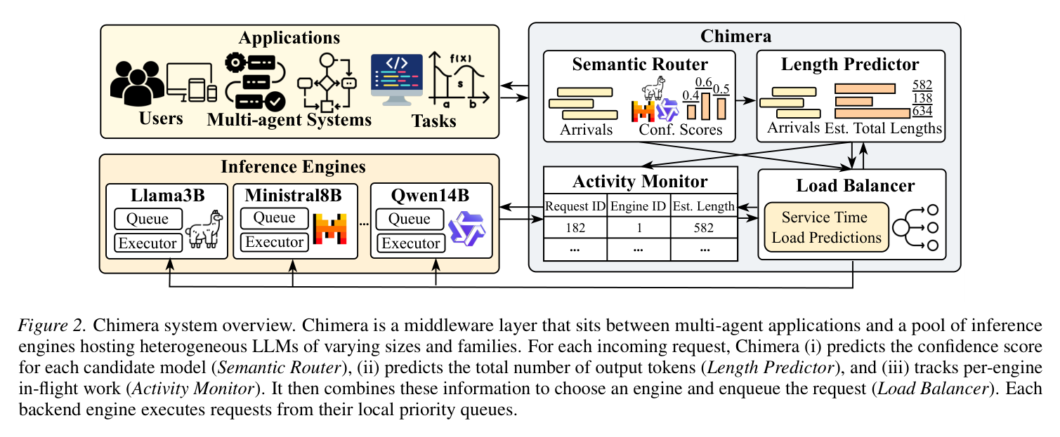
Paper's Figure 2 (caption: "Chimera system overview. Chimera is a middleware layer that sits between multi-agent applications and a pool of inference engines... (i) predicts the confidence score for each candidate model (Semantic Router), (ii) predicts the total number of output tokens (Length Predictor), and (iii) tracks per-engine in-flight work (Activity Monitor). It then combines these information to choose an engine and enqueue the request (Load Balancer). Each backend engine executes requests from their local priority queues.")
The figure makes the division of labor explicit: three cheap predictors feed one dispatcher, and each backend engine owns a local priority queue. Note that the router/predictor sit off the critical path (async batched services); the engines keep doing continuous batching and KV-cache management.
The agent-loop / per-request decision (Algorithm 1) #
Because a workflow is a sequence of stages sharing a program_id, the "loop" here is the scheduler's per-request decision, with model assignment reused across a workflow's stages to preserve KV-cache locality.
The Mermaid captures the branch the raster figure cannot: the assignment-reuse fork at the top. The router (a GPU-occupying transformer) runs only on a workflow's first request; subsequent stages skip routing entirely. Error/overflow recovery is implicit — congested models simply see their $L[m]$ rise and shed traffic (monotone fallback), and starved requests are promoted via aging rather than dropped.
Memory model: short-term = each engine's local priority queue + KV-cache; the "long-term" memory is the offline-trained router weights and QRF, plus the offline-profiled decode_ms_per_token/max_batch_size per model. Episodic state = the Activity Monitor's program table (program_id → assigned engine, remaining length), which is live work-in-flight, cleared on completion.
4. 作者证明 #
无形式化作者证明 — 仅实证. Chimera has no convergence or optimality theorem; all guarantees are empirical Pareto-dominance. What could have been bounded but was not: a queueing-theoretic bound on worst-case wait under the aging mechanism (only claimed to "improve worst-case waiting time"), or a regret bound on model selection vs. the oracle router. The paper instead supplies definitions and an analytical fallback argument.
Notation table:
| Symbol | Meaning |
|---|---|
| $r=(p,i,x_r,\textit{meta}_r)$ | request: program id, stage index, prompt, metadata |
| $N_p$ | number of stages in workflow $p$ |
| $C_p,\ S_p$ | end-to-end completion time; task performance score |
| $q[m]=\sigma(\ell_{r,m})$ | per-model confidence (sigmoid, multi-label) |
| $Y_r=\sum_{j=i}^{N_p}\text{OutTokens}(p,j)$ | total remaining workflow output tokens |
| $\hat{y}\approx\text{median}(Y_r\mid\phi(r),m^\star)$ | predicted priority (conditional median) |
| $P_m=\sum_{t\in\text{Values}(\mathcal{I}[m])}t$ | in-flight predicted tokens on model $m$ |
| $L[m]=\frac{P_m\cdot\Pi[m].\text{decode\_ms\_per\_token}}{\Pi[m].\text{max\_batch\_size}}$ | TTLT estimate |
| $\tau,\ \Delta s$ | latency slack; confidence margin |
| $S,\ Q$ | starvation threshold; running quantum (aging) |
方程物理意义: $q[m]=\sigma(\ell_{r,m})$ uses sigmoid (not softmax) so several models can be simultaneously confident — routing is multi-label, not mutually exclusive. $L[m]$ divides committed token work by batch parallelism × per-token cost, an amortized delay estimate; larger $\text{max\_batch\_size}$ lowers effective delay. Selection $L[m]\le(1+\tau)L_\text{fast}$ AND $q[m]\ge q^\star+\Delta s$ picks fastest by default, upgrades only if a stronger model stays within slack and clears the margin.
6 minimum checks:
- Dimensional check — $L[m]$: tokens × (ms/token) / (dimensionless batch) = ms. ✓ consistent with "TTLT estimate" in ms.
- Monotonicity (load) — as more work admits to $m$, $P_m\uparrow \Rightarrow L[m]\uparrow \Rightarrow$ constraint (i) eventually fails $\Rightarrow$ traffic sheds to less-loaded models. Matches the "monotone fallback" claim.
- Boundary $\tau\to0$ — only models tied for fastest latency are eligible ⇒ latency-first (matches "tighter slack prioritizes lower latency").
- Boundary $\tau\to\infty$ — load constraint always satisfied ⇒ pure highest-confidence routing (performance-first). Matches slack as a tuning knob (§4.3).
- Boundary $\Delta s\to\infty$ — no model ever beats the margin ⇒ always use $m_\text{fast}$; never switches. Consistent with "avoid switching models for marginal gains / promote KV reuse".
- Degenerate homogeneous cluster — all $q[m]$ and $\Pi[m]$ equal ⇒ selection collapses to $m_\text{fast}$ and STJF-by-$\hat{y}$ only; reduces to a length-aware scheduler, sane baseline behavior.
- Assignment reuse across a workflow's stages (Algorithm 1 lines 2, 24–26): the router runs only on a workflow's first request; later stages reuse
A[program_id]. This both saves the GPU-occupying router call and promotes KV-cache reuse — and it means finer per-stage routing is deliberately not attempted. - Async batched predictor/router off the critical path (§3.8): requests enqueue lightweight feature objects; a background collector batches to a max size or timeout; inference runs in a separate process pool so it never contends with the scheduler event loop. The scheduler blocks only on the two minimal outputs (confidence scores, $\hat{y}$) needed for dispatch — this is why overhead stays ≤2.2% despite two learned models in the loop.
Success-rate model (empirical sweep): the $(C,S)$ frontier is swept over (dataset ∈ {APPS,MATH}, RPS ∈ {8,12,16}, model combo ∈ {Qwen1.5+7B, Qwen1.5+14B, Llama3B+Minis8B, Qwen1.5+3+14B}, slack τ). Monotonicity holds along RPS (latency rises with load) and along τ (performance rises, latency loosens). Failure-mode note: the dominant residual bottleneck flips by model combo — oracle predictor helps Qwen1.5+7B (length-prediction error binds under tight latency), oracle router helps Qwen1.5+14B (routing binds). Latency budget per turn: router 0.1–1.1% + predictor 0.1–1.1% of E2E ⇒ scheduler ≤2.2% (Table 1); no per-turn "interactive latency" claim, but the overhead is negligible relative to decode.
5. 实验与数据 #
Main frontier. The load-bearing result is the latency-vs-performance scatter across all combos; Chimera occupies the lower-right (best) region.
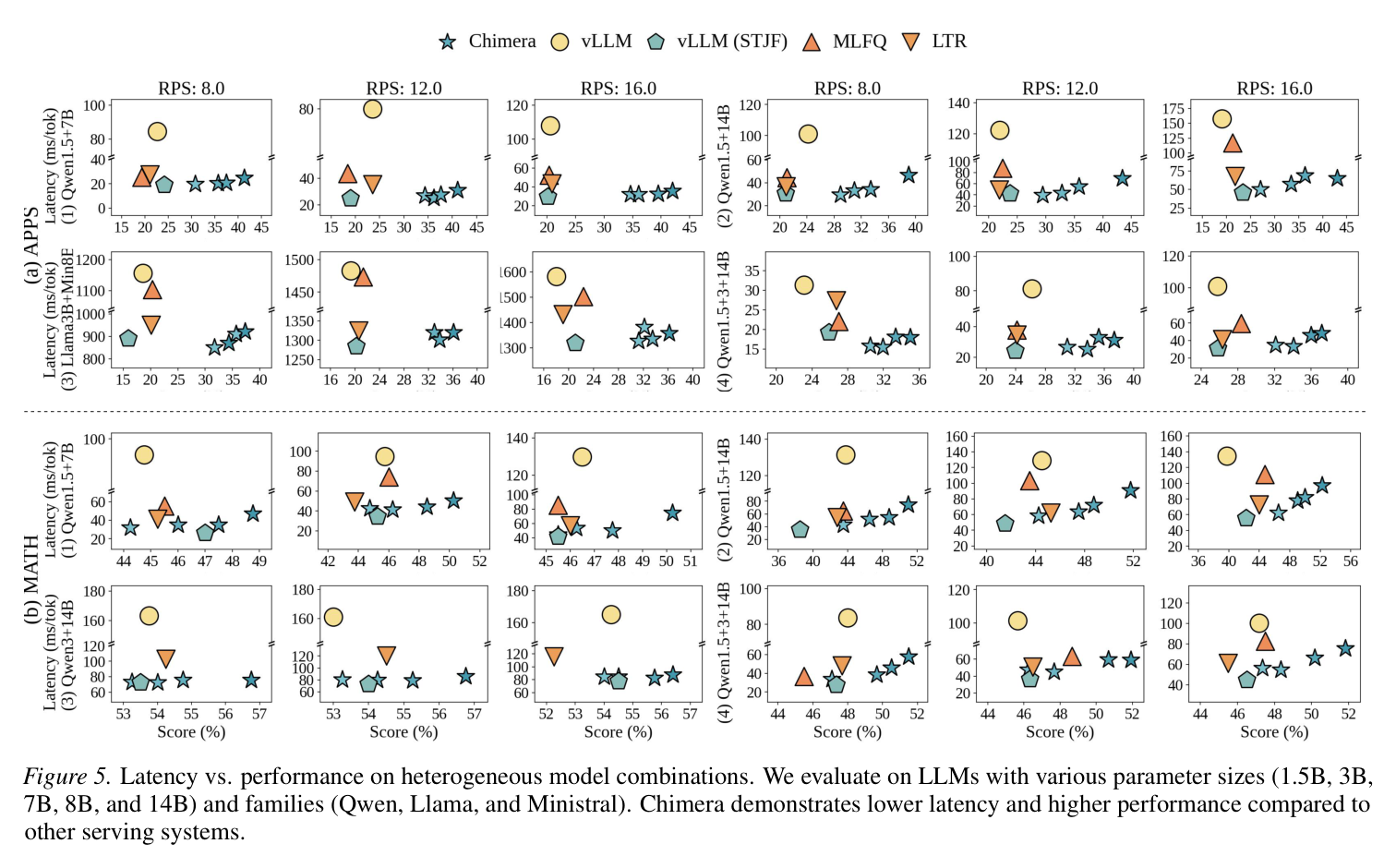
Paper's Figure 5 (caption: "Latency vs. performance on heterogeneous model combinations. We evaluate on LLMs with various parameter sizes (1.5B, 3B, 7B, 8B, and 14B) and families (Qwen, Llama, and Ministral). Chimera demonstrates lower latency and higher performance compared to other serving systems.")
Lower-right is better. Baselines (vLLM, MLFQ, LTR) mostly move left (lower latency) but not up (performance stays flat) — they don't jointly optimize. Chimera moves to the corner and exposes a whole frontier as τ varies. On the hard Llama3B+Ministral8B config Chimera nearly matches vLLM(STJF), the oracle-length reference (both 1.2× over vLLM).
STJF queue-time benefit. The priority policy is validated in isolation on single Qwen models.
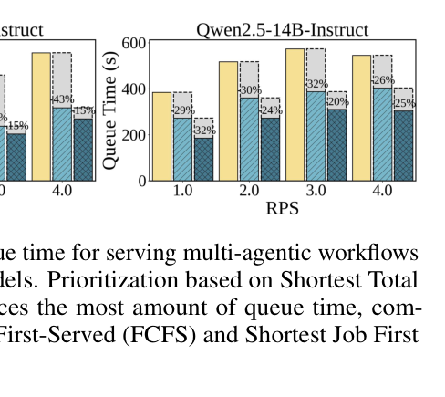
Paper's Figure 3 (caption: "Average queue time for serving multi-agentic workflows with single Qwen models. Prioritization based on Shortest Total Job First (STJF) reduces the most amount of queue time, comparing to First-Come First-Served (FCFS) and Shortest Job First (SJF).")
SJF cuts queue time 26–48% over FCFS; STJF (workflow-aware) adds a further 15–34% over SJF — the incremental win specifically attributable to summing future stage lengths rather than just the current request.
Router ablation. Removing the router collapses query-adaptive selection.
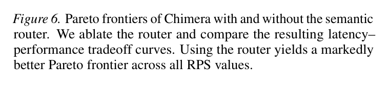
Paper's Figure 6 (caption: "Pareto frontiers of Chimera with and without the semantic router. We ablate the router and compare the resulting latency–performance tradeoff curves. Using the router yields a markedly better Pareto frontier across all RPS values.")
Without confidence scores the system falls back to a fixed heuristic (e.g. "use the stronger model when slack permits") and must pay more latency for the same performance — the router's per-query signal is what bends the frontier.
Heavy-tailed lengths motivate QRF. The distributions justify predicting a median, not a mean.
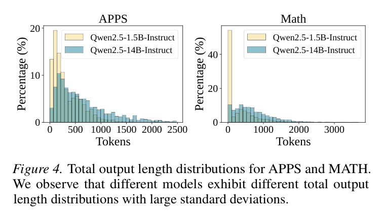
Paper's Figure 4 (caption: "Total output length distributions for APPS and MATH. We observe that different models exhibit different total output length distributions with large standard deviations.")
Std can exceed the mean (APPS Qwen1.5B: mean 447, std 1276; MATH Qwen1.5B: mean 606, std 2587). A conditional-median QRF is robust to these tails, unlike a mean regressor.
Overhead (Table 1): E2E latency 17–79 s; scheduler adds ≤646 ms, i.e. 0.2–2.2% — router and predictor each ≤1.1%. Predictor ranking quality (Table 3): QRF Kendall-τ distance ≈0.12–0.27 (12–27% inverted pairs) vs FCFS ≈0.50 and input-length proxy ≈0.54–0.70; −0.314 over FCFS, −0.371 over input-length. Router (Table 2): ModernBert-large mAP 0.631 avg (APPS 0.521 / MATH 0.740), beating ModernBert-base (0.595).
6. 论证链 #
| # | Step | Support (paper-internal) |
|---|---|---|
| 1 | Multi-agent tasks = multi-stage workflows; E2E latency emerges from cross-stage queueing, so request-level scheduling is suboptimal. | §1 para 3, Figure 1 |
| 2 | Heterogeneous clusters expose a latency–performance trade-off, but model choice and congestion are coupled (routing hard requests to slow models amplifies contention). | §1 para 3 |
| 3 | Therefore evaluate systems by the achievable $(C,S)$ operating-point set (Pareto), not a scalarized objective. | §3.1 objective |
| 4 | To route well you need per-query model confidence ⇒ multi-label sigmoid router; to schedule well you need workflow-total remaining length ⇒ QRF median $\hat{y}$. | §3.3, §3.4 |
| 5 | To couple routing with congestion, estimate per-model TTLT $L[m]$ from in-flight predicted tokens; select highest-confidence model within $(1+\tau)L_\text{fast}$ and margin $\Delta s$. | §3.5, §3.6 |
| 6 | Prioritize by $\hat{y}$ (STJF) with aging so short workflows finish first without starving long ones; STJF cuts queue time beyond SJF. | §3.4 (Fig 3), §3.7 |
| 7 | Empirically this traces the best $(C,S)$ frontier across datasets/RPS/combos at ≤2.2% overhead, near-oracle in hard cases. | §4.3 (Fig 5), Table 1 |
7. 实现 cross-reference #
[实现未公开] — no public code repository is referenced in the source; all citations below are to the paper's own algorithm listing and prose.
核心技术壁垒 (dedicated). The single hardest-to-replicate insight is the workflow-total remaining-length signal $Y_r=\sum_{j=i}^{N_p}\text{OutTokens}(p,j)$ predicted cheaply and used twice. Replicating it requires (a) offline traces labeling each stage's realized output length per model, (b) a per-model QRF conditioned on features {system/user/full token counts, workflow id, stage id, model name, TF-IDF+truncated-SVD text sketch} (Algorithm 1 line 28; §3.4 feature list), and (c) wiring the same $\hat{y}$ into both the priority key and the Activity Monitor's in-flight accounting so the load estimate and the schedule stay consistent. Getting the future-stage sum right (not just current-stage length) is the non-obvious part — it is what separates STJF from ordinary SJF and drives the extra 15–34% queue-time reduction.
关键实现细节 (easy-to-miss tricks):
Tool & environment interface. Tool catalog = the workflow stages (Planner / Coder / QAAggent / Solver / Verifier), each a system-prompted LLM call over the accumulated history; ReAct-style, 1–4 stages (Appendix A.1). Chimera exposes OpenAI-compatible chat/generation endpoints (§3.8), so the environment contract is a stateless request API with the engine owning KV-cache; side effects are confined to code execution against APPS hidden tests (evaluated externally, not by the scheduler).
LLM backbone requirements. Method is backbone-agnostic on the served models (validated across Qwen 1.5/3/7/14B, Llama3.2-3B, Ministral3-8B); the only fixed backbone is the router (ModernBert-large, chosen over base for longer context and higher mAP — §B.1). No CoT/tool-call-format dependency is required of served models beyond producing the workflow stage outputs.