Scepsy: Serving Agentic Workflows Using Aggregate LLM Pipelines
Scepsy: Serving Agentic Workflows Using Aggregate LLM Pipelines — L2 #
1. TL;DR #
Agentic workflows have wildly unpredictable end-to-end latency, but each LLM's share of total execution time is stable. Scepsy exploits this: it traces workflows framework-agnostically, folds them into an "Aggregate LLM Pipeline" (a cheap throughput/latency predictor), then jointly searches fractional GPU shares + tensor-parallel degrees + replica counts, placing them topology-aware on Kubernetes. Up to 2.4× throughput, 27× lower latency.
2. Q1 / Q2 / Q3 #
Q1 — 痛点 (Pain point) #
Serving agentic workflows (multiple LLMs + tools orchestrated to solve a task) on a self-managed GPU cluster is hard for four reasons that compound:
- Arbitrary programs: workflows are written in diverse frameworks (LangChain, LangGraph, AutoGen, Camel) — no single programming model can be assumed.
- Unpredictable execution: token-by-token generation plus data-dependent branching, fan-out, and recursion make per-request latency vary drastically. The paper's beam-search trace shows a single request's generator-LLM invocation count spanning 24–844, and end-to-end latency spanning 9–264 s.
- Conflicting objectives: throughput wants more data-parallel replicas; latency wants more tensor parallelism per replica — they contend for the same GPUs, and adjusting one LLM shifts the bottleneck to another.
- Oversubscribed GPUs: workflows mix heterogeneous LLMs (embedding, generator, reward), and coarse whole-GPU allocations waste capacity in small clusters where every inefficiency is costly.
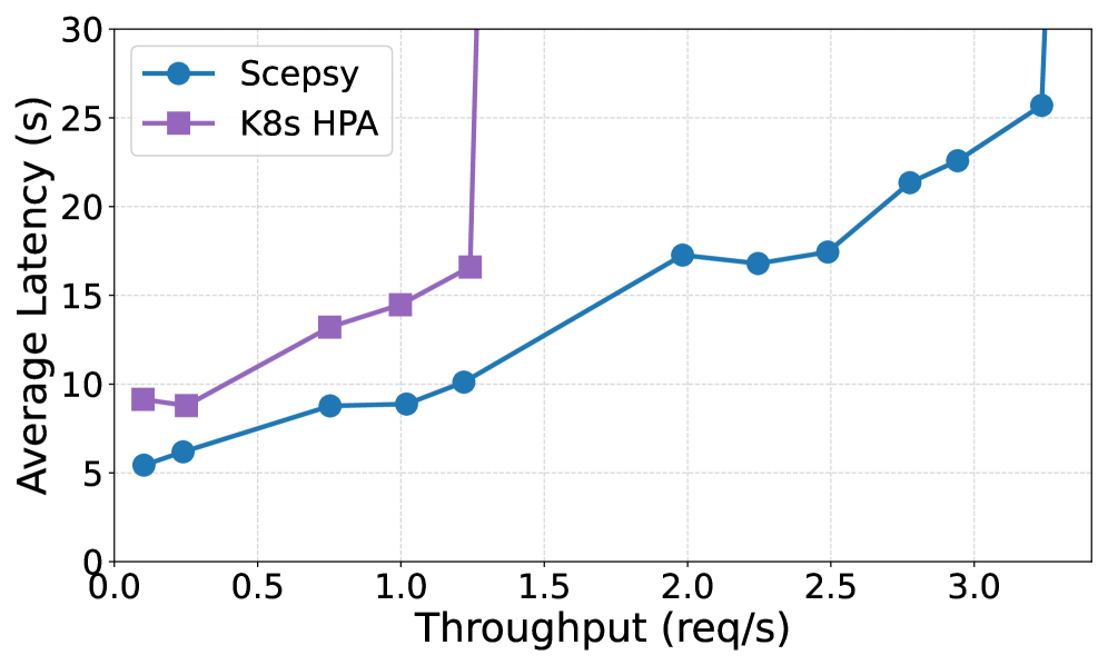
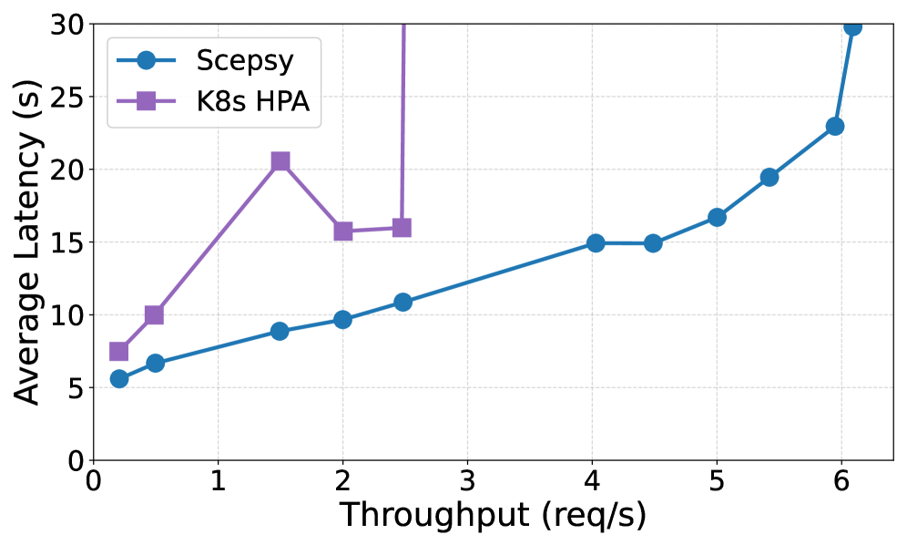
- vs Kubernetes autoscaler: up to 2.4× throughput (beam search, 4 GPU) and 1.4×–27× latency reduction (RAG+reranker, 16 GPU).
- vs Aegaeon (multi-LLM multiplexing): 7.3× throughput / 14.1× latency (beam search, 4 GPU).
- vs Ayo (workflow-aware): up to 8.2× throughput (beam search, 8 GPU); Ayo occasionally wins at a few latency-bound points via request batching.
- Scheduler search stays < 35 s (16 GPU) and ≤ 70 s even at 128 GPU, despite a raw space of ~29 million mappings.
- Memory model: short-term = each LLM's context window; the "long-term" state that Scepsy cares about is the trajectory log (execution traces captured by the HTTP proxy), which is what feeds the aggregate statistics — Scepsy does not itself add vector-DB memory.
- Tool invocation: tools are intercepted only insofar as they interleave LLM calls; Scepsy treats non-LLM code as negligible latency and discards it from the resource model.
- Error recovery: the serving-system recovery path is Kubernetes control-plane restart/health management for a crashed replica; the workflow-level control flow (retry, backtrack over beams) is opaque to Scepsy by design — it only observes aggregate demand.
- Planning style: the workloads Scepsy serves use inference-time scaling — beam search (a bounded tree search over reasoning steps) and RAG+reranker (retrieve → rerank → generate). Scepsy itself does not plan; it schedules.
- Budget: per-workflow arrival rate $\lambda_w$ is the operating knob; the search space bounds are number of LLMs, GPUs, and fractions per GPU.
- Backtracking: at the workflow level, beam search backtracks by pruning beams; at the scheduling level there is no backtracking — the scheduler enumerates and picks the highest-utility feasible allocation once.
- Units: $L_m$ is seconds/request at rate $\lambda_w n_m$; $n_m/p_m$ is dimensionless; product is seconds/workflow-request. ✓ consistent with $L_w$.
- Degenerate $n_m=1, p_m=1$: a single serial LLM gives $L_w = L_m(\lambda_w)$ and $T_w = T_m$ — reduces to single-LLM serving. ✓
- Parallelism limit: if $p_m = n_m$ (all invocations fully parallel), the latency scale factor is 1, i.e., the LLM contributes only one request's worth of latency. ✓ physically sensible.
- Replica scaling (§4 Step ⑤): $d_m$ replicas rescale the arrival rate to $\lambda_w n_m / d_m$ — consistent with the stated assumption that throughput scales linearly with replicas and latency is replica-independent.
- Monotonicity: $L_m(\cdot)$ is increasing in arrival rate (measured latency rises toward saturation), so higher $\lambda_w$ raises $L_w$ — matches the throughput–latency curves rising to the right in Fig. 6.
- Bottleneck consistency: the LLM achieving the min in Eq. 2 is the throughput bottleneck; giving it more replicas raises its $T_m$ and can move the min to another LLM — this is exactly the "shifting bottleneck" the scheduler must chase. ✓
- Success-rate / sweep: this is a serving paper, so the "success" axis is served throughput at target latency, swept over (workload, cluster size 4/8/16 GPU, baseline). Monotonicity: Scepsy dominates all baselines across all cluster sizes; the margin over Kubernetes is non-monotonic in GPU count (2.4× at 4 GPU, 1.5× at 8, 1.8× at 16 for beam search), reflecting allocation-granularity effects.
- Latency budget per turn: per-turn cost = LLM inference + negligible tool/orchestration (claimed few ms). No claim of fixed "interactive latency"; instead the pipeline predicts a latency curve vs. arrival rate.
- Failure-mode classification: §9 identifies exactly three model-breaking cases — (1) fan-out across different LLMs mis-modeled as serial, (2) bimodal load when an LLM is reused in distinct roles, (3) non-negligible long-running tools. The dominant assumption-violation is (3), which the negligible-tool-time claim directly depends on.
- Tracing: implemented as an HTTP proxy in front of each LLM engine's completions API — captures request/response contents + timestamps + workflow id (§4 Step ①). Framework-agnostic by construction.
- Serving stack: one vLLM or SGLang engine per replica; one SGLang router per workflow for load- and KV-cache-aware routing (§6 Para 4).
- Placement enforcement: Scepsy emits Kubernetes deployment files that lock inter-node placement, plus an extended Nvidia device plugin for intra-node GPU-fraction placement; Nvidia MPS with static SM/memory limits enforces per-fraction isolation (§6 Para 4).
- Contiguous-only fraction packing as a symmetry-pruning device (§5 Step ①–②): by allocating GPUs only contiguously and packing the highest-latency LLM's fraction as a whole GPU first (1.66 GPUs → 1.0 + 0.66), Scepsy both minimizes partitioning of latency-critical LLMs and collapses equivalent permutations, which is a large part of why the ~29M space becomes searchable. It is a scheduling correctness detail masquerading as a performance detail.
- Latency-ratio ordering to bound per-LLM fractions (§5 Step ①): each LLM's lower bound is the fractions needed just to load params + KV cache; its upper bound subtracts the minimum fractions of all lower-latency LLMs. This ordering-derived bound is what excludes nonsensical allocations (small embedding LLM out-resourcing a large generative LLM) without an explicit constraint solver.
Existing systems fail on a subset: workflow-aware systems (Parrot, Ayo, Autellix) are single-LLM and/or framework-restricted and leave GPU allocation to the user; multi-LLM systems (AlpaServe, MuxServe, Prism, Aegaeon, Kubernetes autoscaling) schedule each LLM in isolation with no workflow awareness. No prior system has all four properties simultaneously.
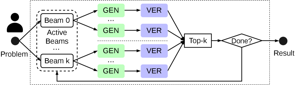
Paper's Figure 1, verbatim (caption: "Beam search as an agentic workflow (Beam search uses inference-time scaling, which uses LLMs to explore multiple reasoning paths as a search tree.)"). This is the running motivating workload: a small generator LLM (GEN) proposes candidate reasoning steps, a larger verifier LLM (VER) scores them, and only the top beams survive — producing exactly the multi-LLM, heterogeneous-size, fan-out/fan-in pattern that isolated-LLM schedulers cannot reason about.
Q2 — 方法 (Method) #
Scepsy is an orchestration layer between agentic frameworks and LLM engines. It runs four stages: (①) trace LLM-level requests via an HTTP proxy in front of each engine's completions API (framework/engine-agnostic); (②) fold the trace into an Aggregate LLM Pipeline using two per-LLM statistics — average invocations per request $n_m$ and average request-level parallelism $p_m$ — plus replay-based per-LLM throughput/latency profiles; (③) a GPU scheduler searches a pruned space over fractional GPU shares, tensor-parallel degree, and replica count for each LLM, using the pipeline as a fast predictor; (④) a topology-aware placement heuristic maps fractions onto GPUs respecting NVLink domains, deployed via Kubernetes + Nvidia MPS.
核心技术壁垒 (THE single hardest-to-replicate insight): the decision to abandon modeling control flow entirely. Instead of predicting when/whether a branch or loop fires (what prediction-based schedulers attempt and where they break for multi-LLM), Scepsy reasons only about the aggregate fraction of demand each LLM bears. This works because the relative per-LLM time shares are empirically ~4× more stable than absolute latencies (Fig. 3). Two scalar statistics ($n_m$, $p_m$) captured from timestamp overlaps then suffice to bridge LLM-level and workflow-level load without any static analysis of the workflow. Reproducing this requires trusting — and empirically validating on your own workloads — that steady-state aggregate shares are stable, which is counter-intuitive given the extreme per-request variance.
Q3 — 结果 (Results) #
On a 16-GPU on-prem cluster (4 nodes × 4 RTX A6000) with RAG+reranker and beam-search workloads:
3. 架构 / 方法图 #
The system is a four-stage pipeline (Fig. 2), and the core abstraction — the Aggregate LLM Pipeline — is built in five steps (Fig. 4).
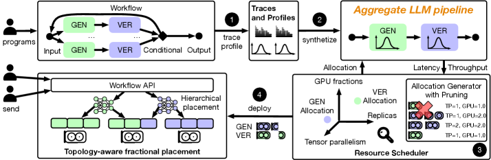
Paper's Figure 2, verbatim (caption: "Scepsy Overview"). The reader should notice the aggregation act at the center: the looped and parallel per-request LLM invocations on the left collapse into two ordered stages (GEN, VER) on the right. This is why the term "pipeline" is slightly misleading — stage ordering does not matter for the prediction (§4); it is really an aggregate resource model that borrows pipeline throughput/latency math.
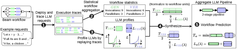
Paper's Figure 4, verbatim (caption: "Construction of an Aggregate LLM Pipeline for beam search workflow"). The five steps are: (1) workflow tracing → (2) statistical aggregation into $n_m$, $p_m$ → (3) per-LLM profiling by trace replay at varying arrival rates and TP degrees → (4) synthesis into workflow-level throughput/latency curves → (5) prediction for any candidate allocation. Notice non-LLM tool/orchestration time is discarded here (assumed negligible, "at most a few milliseconds").
Because the target is an agent-serving system, the per-request agent loop is what generates the load being aggregated:
Planning & reasoning (of the served workloads) #
4. 作者证明 #
无形式化作者证明 — 仅实证. Scepsy provides an analytical predictor (Eqs. 1–2) but no formal guarantee that the predictor is accurate, that the pruned search finds the optimum, or that aggregate shares remain stable — all three rest on empirical evidence. This matches the agent-serving norm: the load-bearing "proof" is that relative statistics are ~4× more stable (Fig. 3) and that predictions match measured throughput/latency curves (Fig. 6–8). The metric that could have been bounded is prediction error vs. ground-truth profiling, but the paper reports it only implicitly through end-to-end curve fit.
Notation table #
| Symbol | Meaning |
|---|---|
| $\lambda_w$ | target workflow-level arrival rate |
| $\lambda_m$ | induced LLM-level arrival rate, $\lambda_m = \lambda_w \cdot n_m$ |
| $n_m$ | average invocations of LLM $m$ per workflow request |
| $p_m$ | average request-level parallelism of LLM $m$ (overlapping-timestamp count) |
| $L_m(\cdot)$ | average per-request latency of LLM $m$ at a given arrival rate |
| $L_{w_m}$ | workflow-level latency contribution of LLM $m$ |
| $L_w(\lambda_w)$ | total workflow latency at $\lambda_w$ |
| $T_m$ | maximum sustainable throughput of LLM $m$ |
| $T_w$ | maximum workflow throughput |
| $TP_m$, $d_m$ | tensor-parallel degree and replica count for LLM $m$ |
方程物理意义 #
Workflow latency accumulates along the per-request critical path:
$$L_{w}(\lambda_{w})=\sum_{m}L_{w_{m}}(\lambda_{w})=\sum_{m}L_{m}(\lambda_{w}\cdot n_{m})\cdot\frac{n_{m}}{p_{m}}$$
Each LLM's latency is evaluated at its induced arrival rate $\lambda_w \cdot n_m$, then scaled by $n_m/p_m$ — multiply by how many times the LLM runs per request, divide by how many of those run in parallel. Summation (not max) is used because stages accumulate along a single request's critical path.
Workflow throughput is bottleneck-limited:
$$T_{w}=\min_{m}\frac{T_{m}}{n_{m}}$$
The slowest stage (min over LLMs of sustainable throughput divided by per-workflow invocation count) caps the whole workflow. Parallelism $p_m$ and $\lambda_w$ drop out here — parallel requests do not reduce an LLM's total request count, and max throughput is independent of arrival rate.
6 minimum checks #
Agent-specific asks #
5. 实验与数据 #
Cluster: 16 GPUs (4× RTX A6000 per node, 100 Gbps InfiniBand, NVLink in GPU pairs). Engines: vLLM v0.17 + SGLang router (v0.2/v0.2.2 for the Ayo comparability run). Workloads: RAG+reranker (e5-base-v2 + Llama-3-8B) and beam search (Llama-3.2-1B generator + Llama-3.1-8B-PRM verifier).
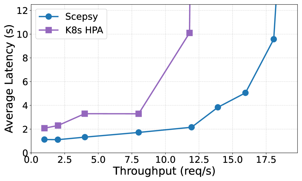
Paper's Figure 6, verbatim (caption: "Throughput–latency comparison across workloads and 4, 8, 16 GPUs"). This is the headline figure: x = achieved throughput, y = workflow latency, one panel per (workload × cluster size). Scepsy's curve sits below-and-right of Kubernetes everywhere. Kubernetes oscillates (scales up, empties queues, scales down) and cannot exploit tensor parallelism — the source of the up-to-27× latency gap. This figure is where the 2.4× / 27× headline numbers come from.
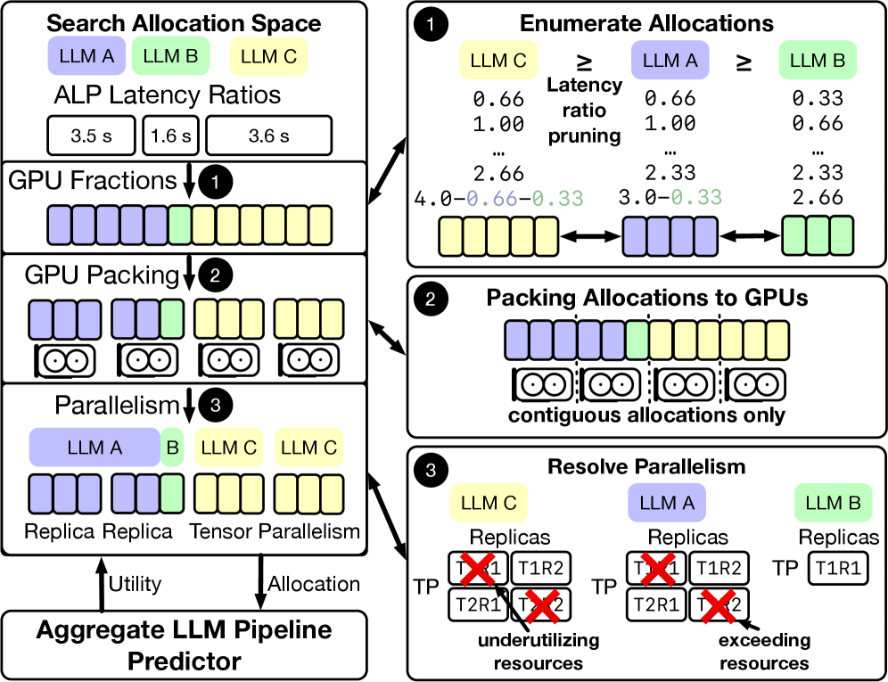
Paper's Figure 5, verbatim (caption: "Overview of GPU scheduling in Scepsy"). The scheduler's pruned search: (①) enumerate LLM→GPU-fraction mappings ordered by latency ratio, (②) pack fractions contiguously onto physical GPUs (e.g. 1.66 GPUs → 1.0 on GPU 1 + 0.66 on GPU 2), (③) resolve feasible TP × replica combinations (must evenly divide the GPU count; TP capped at the high-bandwidth interconnect degree). This is what keeps a ~29M-mapping space searchable in seconds.
Paper's Figure 10, verbatim (caption: "Ablation study showing the contribution of Scepsy's key optimizations across workloads and cluster scales"). The load-bearing attribution result: for RAG+reranker, co-location (fractional GPUs) is the biggest throughput contributor (heterogeneous small embedding + large generative LLM benefits most from sub-GPU packing); for beam search, tensor parallelism drives the latency reduction. Disabling both compounds the degradation — the two mechanisms are synergistic, not redundant.
Paper's Figure 11, verbatim (caption: "Search time as scheduling parameters scale for the combined workflow"). Three panels show search time growing exponentially in LLM count and GPU count yet staying practical: < 35 s across LLM counts (16 GPU, 10 fractions), ≤ 70 s at 128 GPU, ≤ 1 s across fractions-per-GPU. This validates the §5 pruning strategies — without them the raw ~29M-mapping enumeration would be intractable.
The distribution figures (Fig. 3a absolute, Fig. 3b relative) are the empirical crux motivating the whole design — absolute per-LLM latencies over 500 beam-search requests are widely spread, whereas relative time shares are up to 4× tighter, justifying allocation by aggregate share rather than absolute prediction.
6. 论证链 #
| Step | Claim | Support (paper-internal) |
|---|---|---|
| 1 | Agentic workflows have unpredictable absolute latency but stable relative per-LLM time shares | Fig. 3(a) vs 3(b) over 500 beam-search requests; relative up to 4× more stable (§2.4) |
| 2 | Therefore workflow performance can be modeled without control-flow prediction, using only aggregate per-LLM demand | Two statistics $n_m$, $p_m$ from trace timestamps capture loops/branches/fan-out (§4 Step ②) |
| 3 | An Aggregate LLM Pipeline built from these statistics + per-LLM profiles predicts end-to-end throughput/latency cheaply | Eqs. 1–2 reduce prediction to profile lookups + arithmetic (§4 Step ⑤, closing para) |
| 4 | A pruned search over fractional shares + TP + replicas finds a good allocation in seconds | 3 pruning strategies shrink ~29M mappings; search < 35 s / ≤ 70 s (§5 Step ①, §7.5) |
| 5 | Topology-aware placement realizes the allocation without cluster fragmentation | Most-constrained-first heuristic + MPS on Kubernetes (§6) |
| 6 | The full pipeline yields large end-to-end gains vs isolated-LLM and workflow-aware baselines | Up to 2.4× throughput / 27× latency vs Kubernetes; 7.3× / 8.2× vs Aegaeon / Ayo (§7.2) |
| 7 | Both co-location and parallelism are individually necessary | Ablation: co-location dominant for RAG throughput, TP dominant for beam-search latency (§7.4, Fig. 10) |
7. 实现 cross-reference #
[实现未公开] — the prototype (25K lines of Python, "available post-acceptance at https://github.com/anon/Scepsy") is anonymized and not accessible at ingest time, so no file:line citations are possible.
关键实现细节 (easy-to-miss tricks):
核心壁垒 recap: the replicable engineering is standard (proxy tracing, MPS, Kubernetes); the non-obvious, hard-to-replicate bet is that discarding all control-flow modeling in favor of two aggregate scalars ($n_m$, $p_m$) is sufficient to schedule dynamic workflows — validated only empirically by the relative-stability observation (Fig. 3), and explicitly bounded by the three §9 failure modes.