Idleness is Relative — MORI (L2) #

1. TL;DR #

Agentic programs alternate between busy phases (bursts of short tool calls) and idle phases (blocked on a long tool call). MORI ("Memory Offloader with Relative Idleness") reconstructs each live program's idleness $\iota$ from step timing, ranks all programs on a continuous spectrum, keeps the busiest in GPU HBM and spills the most idle to CPU DRAM, slides the tier boundary to fit any GPU:CPU capacity ratio, and enforces admission control at both tiers by simply filling each to capacity — yielding 20–71% higher throughput and 18–43% lower TTFT than the best offloading baseline (TA+O).

Name-collision caution (analysis, for downstream disambiguation). This paper's "MORI" = Memory Offloader with Relative Idleness, an agent-serving KV-cache scheduler. It is distinct from ROCm-mori (an AMD RDMA communication library) and from the repo-local mori-scheduler (a routing/scheduler system). Do not conflate the three; they share only a name.

2. Q1 / Q2 / Q3 #

Q1 — 痛点. Serving agentic (ReAct-loop) workloads accumulates per-program KV cache across tool-call steps that quickly exceeds GPU HBM, forcing offload to CPU DRAM. Tool-call durations vary by 3+ orders of magnitude and are unpredictable, so re-placing KV on every call is impractical: the transfer cost is linear in KV size and can exceed a short gap entirely. Existing policies are phase-blind on two axes:

• Recency/frequency (LRU) evicts the least-recently-active program regardless of whether it is about to resume — it may evict a busy program momentarily in a short gap while retaining an idle program that just entered a minutes-long tool call.
• Static context-length eviction (ThunderAgent) has the same blindness plus a size bias: it may keep a long-context idle program resident and evict a short-context busy one.
• A binary busy/idle label also fails structurally: the busy:idle demand ratio drifts continuously as programs switch phases and grow contexts, and rarely equals the hardware's fixed GPU:CPU capacity ratio (e.g. 1:1.6 vs 1:3.1 depending on DRAM), so one tier is oversubscribed (forced evictions) while the other sits underused (wasted memory).
• Prior offloading systems also lack CPU-side admission control: over-offloading makes idle programs evict each other in DRAM, re-introducing thrashing at the CPU tier.

Q2 — 方法. Define each program's idleness $\iota$ as the fraction of recent wall-clock time spent Acting (in tool calls) vs. total (Acting + Reasoning) over a sliding window of the last $k{=}5$ inference–tool-call cycles (Eq. 1). Rank all active programs on this continuous spectrum and run a sticky control loop (default 5 s tick) that demotes the highest-$\iota$ programs down the tier stack (GPU→CPU→Waiting) and promotes the lowest-$\iota$ programs back up, filling each tier exactly to its physical capacity — which is precisely what enforces per-tier admission control. Placement is propagated to the engine as typed offloading hints (busy / idle / inactive) whose priority order is reversed per tier on top of LRU. In multi-replica mode, an affinity-aware balancer routes a returning program back to the replica that already holds its cache — on GPU or in that replica's CPU DRAM.

• 核心技术壁垒: reframing idleness from an absolute/binary label into a continuous, relative ranking whose partition boundary auto-adapts to any GPU:CPU capacity ratio — no per-hardware tuning — and which unifies GPU-tier and CPU-tier admission control into a single sort-and-fill operation.

Q3 — 结果. At 80 concurrent programs (DP=1): 20–71% higher output throughput and 18–43% lower TTFT than TA+O (the best offloading baseline), 1.6–2.1× throughput and up to 2.8× lower TTFT vs non-offloading systems (SMG/TA). DP=3: 54–79% higher throughput than TA+O while sustaining 99%+ GPU utilization (vs 59–76% for phase-oblivious schedulers that suffer throughput collapse at high concurrency). Program churn drops from 14–15% of programs (0.35–0.38 switches/program) to 0.3–2.9% (0.00–0.04 switches/program).

3. 架构 / 方法图 #

3.1 Agent scope #

• Task class: open-ended coding agents (Claude Code / Codex / Cursor), ReAct-style dynamic workflows — explicitly not the fixed-graph / function-calling regime that Parrot/Teola/Ayo/KVFlow target.
• Interaction pattern: multi-turn, long-horizon (tens of inference steps interleaved with tool calls over minutes per session), with monotonically growing KV cache due to prefix dependencies.
• Autonomy: fully autonomous with occasional human-in-the-loop tool calls (approval waits are one source of idle phases). MORI itself is infrastructure and needs only a program_id per request — no phase hints, no workflow graph from the client.

3.2 System overview #

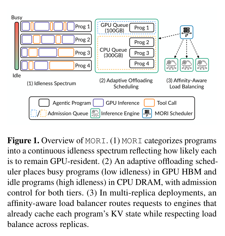
Paper's Figure 1: MORI (1) categorizes programs on a continuous idleness spectrum, (2) an adaptive offloading scheduler places busy (low-$\iota$) programs in HBM and idle (high-$\iota$) programs in DRAM with two-tier admission control, and (3) an affinity-aware balancer routes to engines that already cache each program's KV state. This figure is the load-bearing summary: the three numbered stages map exactly to the idleness metric, the tiering policy, and the multi-replica router — the three contributions.

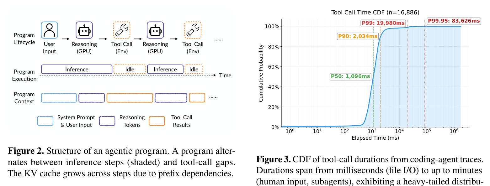
Paper's Figure 2: a program alternates shaded inference steps with tool-call gaps; the KV cache grows monotonically because each invocation shares the prefix of all preceding ones. This is the unit-of-scheduling premise: the gap is inside one logical execution, so the cache stays valuable during it — which is exactly why offloading (preserve on CPU) rather than eviction (discard) is the right primitive.

3.3 The three-tier queue and its mechanics #

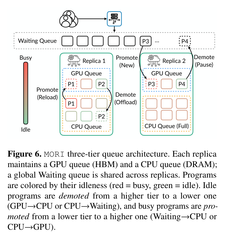
Paper's Figure 6: each replica maintains a GPU queue (HBM) and a CPU queue (DRAM); a single global Waiting queue is shared across replicas. Programs are colored by idleness (red = busy, green = idle); idle programs are demoted downward (GPU→CPU or CPU→Waiting) and busy ones promoted upward (Waiting→CPU or CPU→GPU). This is the structural core of the deepen pass, so the three tiers deserve precise mechanics:

• GPU queue (HBM) — holds programs currently classified busy; requests forward straight to the engine. Invariant: aggregate KV of GPU-queue programs on a replica ≤ GPU capacity.
• CPU queue (DRAM) — holds idle programs; KV is offloaded to the same node's DRAM. Incoming requests are gated until the program is promoted back and its KV reloaded over PCIe. A symmetric DRAM capacity constraint is enforced. Because it is per-replica, the CPU queue doubles as an affinity anchor: a promoted program returns to the replica that already holds its cache and reloads locally instead of recomputing.
• Waiting queue (no cache) — the only global queue; KV has been discarded entirely, so promotion requires a full-prefill recompute. Overflow from both finite tiers lands here.

Admission control as an emergent property (analysis). There is no separate admission module: because tiers are ranked and filled exactly to physical capacity from the busiest end, the act of filling is the admission control. Excess spills one tier down. This is why the design generalizes to any capacity ratio without tuning — the boundary is wherever the cumulative KV footprint of the sorted programs crosses the tier's byte budget.

3.4 The agent-loop state model #

One turn cycles through two instantaneous statuses whose sustained pattern defines the phase (Reasoning = executing on GPU; Acting = blocked on a tool call, KV sitting idle). Every request flips a program to Reasoning; every completed response flips it back to Acting. A busy-phase program rapidly ping-pongs between the two; an idle-phase program stays Acting for a long stretch.

• Memory model: short-term = KV cache in HBM (busy); "long-term" spill = KV in per-replica CPU DRAM (idle, affinity-preserving); discarded = Waiting queue (recompute via full prefill). "Memory" here is only the KV working set — there is no vector-DB / episodic store.
• Tool invocation: opaque to the scheduler; a tool call simply flips the program to Acting for an unknown duration. Parallel tool calls collapse into one gap = max of the individual durations. A spawned subagent is a separate program; from the parent's view its whole execution is one long tool call (idle window).
• Error recovery / fallback: if a program fits neither GPU nor CPU, it falls to Waiting and loses its cache (recompute on resume). Scheduler-gated (queued) time is excluded from $\iota$, so the scheduler's own delays never pollute the phase signal it reads back.

3.5 Where the idleness signal comes from (analysis) #

The paper computes $\iota$ from per-step Reasoning/Acting durations tracked in the router. Framed as a measurement recipe, $\iota$ is reconstructable at a gateway/proxy from just three timestamps per step: forward-to-LLM = Reasoning start; stream-end = Acting start; next-request arrival = Acting end. The subtle correctness requirement (called out in §4.1) is that any scheduler-imposed wait — gating while queued in CPU/Waiting, or KV reload latency — must be excluded from both $T_{\text{reasoning}}$ and $T_{\text{acting}}$; otherwise the metric feeds the scheduler's own queuing delay back into placement and $\iota$ is biased toward "idle," creating a feedback loop that would strand a busy program in a lower tier.

4. 作者证明 #

无形式化作者证明 — 仅实证. As is typical for agent-serving systems, there are no convergence or optimality guarantees. The only formal object is the idleness definition (Eq. 1); everything else is validated empirically across a hardware/model/concurrency sweep.

Notation table #

The one equation and its physical meaning #

$$\iota = \frac{T_{\text{acting}}^{(k)}}{T_{\text{reasoning}}^{(k)} + T_{\text{acting}}^{(k)}}$$

$\iota$ is the fraction of recent time a program left its KV cache sitting idle in HBM while blocked on tools. $\iota \to 1$ = idle phase (offload it); $\iota \to 0$ = busy phase (keep it GPU-resident). Critically it is a proxy for wasted HBM, not a duration prediction — MORI never predicts individual tool-call lengths. The window gives two properties the paper leans on: responsiveness (an ongoing long call's elapsed time keeps growing and soon dominates the window, so $\iota$ rises within a cycle or two of a phase change) and robustness (a single anomalous long call inside a busy burst is diluted by the other $k{-}1$ short cycles, preventing premature reclassification). $k{=}5$ balances these.

6 minimum checks #

1. Success-rate / performance sweep — swept over (GPU tier × model size × concurrency × CPU:GPU ratio): {H200-80GB/7B, H200/30B-MoE, B200/70B-TP2} × {20, 50, 80 programs} × {1×, 2× CPU}. Monotonicity: MORI throughput rises monotonically with concurrency on B200 (136→191→189 tok/s) where TA+O is non-monotonic (147→181→146). The gain over TA+O widens with memory pressure (+2% at 20 programs → up to +71% at 80).
2. Latency budget per turn — TTFT decomposes into queue + KV reload + prefill; MORI's GPU queue prioritizes already-resident programs, cutting reload stalls. No interactive-latency claim at 80 programs (TTFT 33–38 s on B200), but MORI is the lowest of all systems and is the only one that converts extra DRAM (1×→2×) into a TTFT drop (38→33 s) while TA+O stays flat (56→58 s).
3. Failure-mode classification — the paper isolates three baseline failure classes: (a) phase-blind eviction (LRU / context-length keeps idle caches on GPU), (b) uncoordinated CPU LRU (extra DRAM gives TA+O no benefit because HiCache manages it without scheduler coordination), (c) affinity break on eviction (offloading-agnostic router re-routes an evicted program, discarding the CPU-resident cache → cross-replica churn). MORI targets all three; (a) dominates under load and drives the DP=3 throughput collapse.
4. Backbone sensitivity — method is backbone-agnostic (7B Qwen-2.5, 30B Qwen-3 MoE, 70B Llama-3.1 all benefit); it depends on timing behavior, not model capability.
5. Overhead check — Table 2: MORI adds ~2.3 ms CPU scheduling per step (21.5→23.8 ms) but this is fully overlapped with the ~32 ms GPU step, so zero critical-path cost.
6. *What could have been bounded* — the reload-vs-recompute cost tradeoff could be formalized (transfer cost linear in KV size vs. gap duration), giving a competitive-ratio-style bound; the paper argues it informally in §3.2 instead of proving it.

5. 实验与数据 #

Workload: 186 replayed Claude Code traces (of 200 attempted) on SWE-bench Pro (claude-sonnet-4-6, high effort), reconstructed as (input len, output len, tool-call duration) tuples and replayed closed-loop for 1 hour per run. Baselines: SMG (SGLang model gateway, prefix-aware; reduces to direct forwarding at DP=1), TA (ThunderAgent, program-aware, no offload), TA+O (TA + uncoordinated HiCache CPU offload — the strongest baseline).



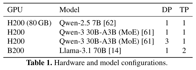
Paper's Table 1: three GPU configs — H200-80GB/7B, H200/30B-MoE (DP=1 and DP=3), B200/70B-TP2. The sweep deliberately spans a loose regime (7B leaves ample KV room) to the tightest (70B TP=2), so the widening MORI advantage tracks memory pressure rather than one lucky config. H200-80GB emulates H100-class capacity by capping HBM (near-identical compute, differing mainly in HBM size/bandwidth).



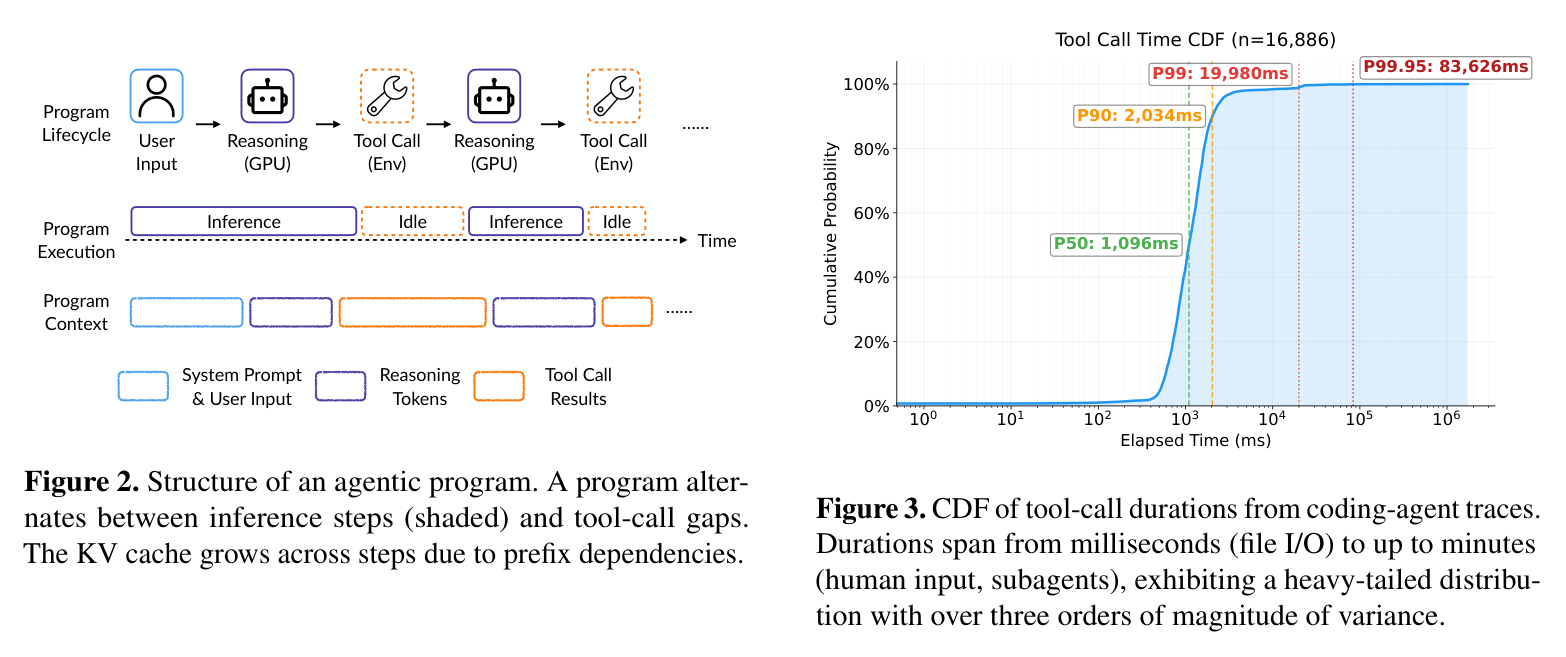
Paper's Figure 3: tool-call durations span sub-second file I/O to minutes (human input / subagents). This heavy tail is the entire motivation: per-call duration is unpredictable and spans decades, so per-call placement is hopeless and a coarser phase-level signal is required.



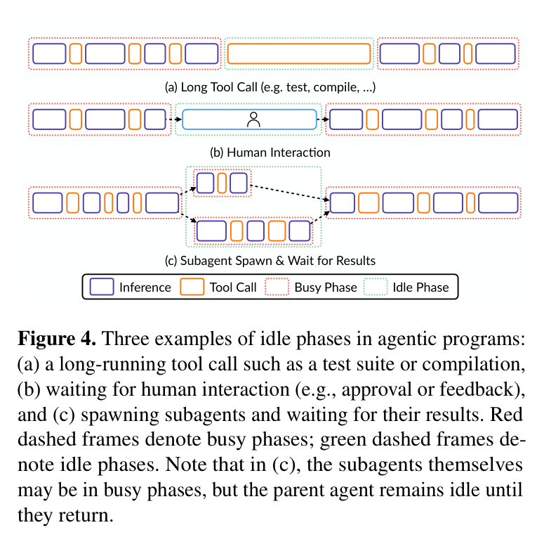
Paper's Figure 4: idle phases arise from (a) a long-running tool call (test suite / compile), (b) waiting for human approval, and (c) spawning subagents. Red frames = busy, green = idle; note in (c) the subagents may be busy while the parent stays idle. This justifies treating a subagent's whole lifetime as one long parent-side tool call — the offload opportunity is precisely these green windows.



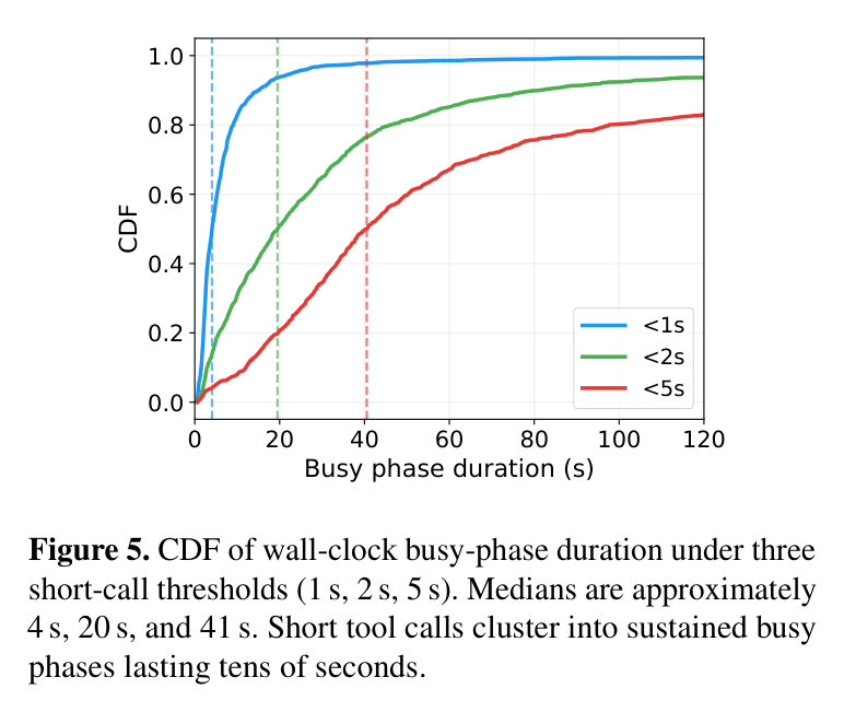
Paper's Figure 5: median busy-phase durations ~4 s / 20 s / 41 s across thresholds; robust to threshold choice. Load-bearing evidence that phases persist (median 20 s at the 2 s threshold; p90 ≈ 81 s), long enough that sticky placement won't oscillate — and that 13% of long calls hold 58% of tool-call wall-time. Phase persistence + identifiability-from-history are the two properties that make $\iota$ a usable scheduling signal.



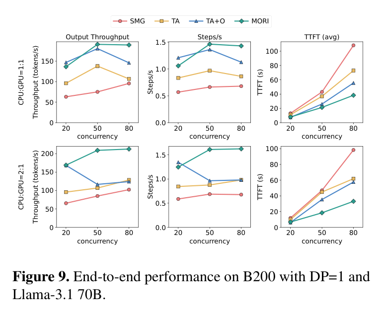
Paper's Figure 9: the tightest memory regime; TA+O throughput is non-monotonic (collapses at 80 programs) while MORI grows monotonically and reaches the largest relative gain (+71%). This is the case-study config: eviction thrashing is unavoidable here, so it most cleanly separates phase-aware from phase-oblivious placement. TTFT here is 38 s (MORI) vs 56 s (TA+O), 73 s (TA), 108 s (SMG) — a 2.8× reduction over SMG.



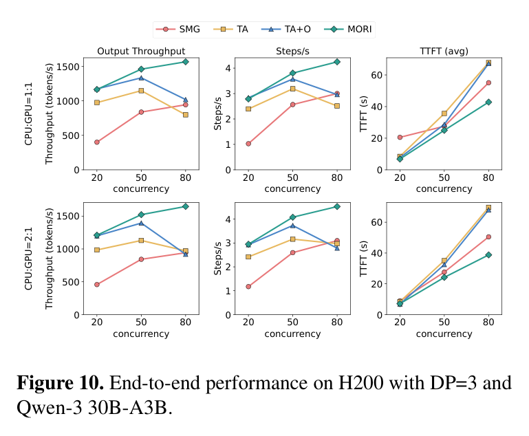
Paper's Figure 10: multi-replica setting; MORI sustains 99%+ GPU utilization and 54–79% higher throughput while phase-oblivious baselines collapse (TA falls 1147→798 tok/s as concurrency rises 50→80). The DP=3 story is really about affinity: TA/TA+O maintain only GPU-level affinity, so an evicted program is treated as cacheless and re-routed to the lightest-loaded replica — even though its KV still sits in the original replica's DRAM — forcing a full recompute. MORI tracks residency across both GPU and CPU tiers and routes the returning program home, cutting churn from 14–15% to 0.3–2.9% and letting memory tiering and cross-replica load balancing be co-optimized rather than traded off. (Contrast SMG's prefix-only affinity, which under pressure concentrates traffic on one replica — 13.8 running reqs vs 1.4/1.5 on the others — for just 51% utilization.)

Overhead detail. Table 2 (H200 / 30B / DP=1): TA+O ~29 ms GPU step, 21.5 ms CPU; MORI ~32 ms GPU step, 23.8 ms CPU. Both finish scheduling before the GPU step ends (margins 7.6 ms and 8.6 ms), so MORI's richer logic adds no critical-path latency.

Honest tie. At 20 programs on H200-80GB / 1× CPU, MORI 546 vs TA+O 534 tok/s (+2%) — when the working set fits in CPU, phase-awareness is marginal and both hit 87–96% cache hit rates.

6. 论证链 #

Step	Claim	Support (paper-internal)
1	The scheduling unit is the program, not the request; its KV cache grows and stays valuable across tool-call gaps.	§3.1 + Fig. 2 (prefix dependencies, monotone KV growth).
2	Per-call tool durations are unpredictable and heavy-tailed, so per-call placement is impractical (transfer cost can exceed a short gap).	§3.2 + Fig. 3 (3+ orders of magnitude variance).
3	But at program granularity, behavior clusters into persistent busy/idle phases identifiable from recent history.	§3.3 + Fig. 4, Fig. 5 (median 20 s busy phases; 13% long calls = 58% of tool time).
4	A binary busy/idle label can't match a fixed GPU:CPU capacity ratio; LRU/context-length eviction is phase-blind; CPU tier also needs admission control.	§3.4 (three challenges).
5	Therefore idleness must be a continuous, relative ranking $\iota$ that slides the partition boundary to hardware and fills each tier to capacity (= admission control).	§4.2 Eq. 1 + §4.3 sticky ranking + demotion/promotion rules.
6	Ranking-driven placement + typed reversed-LRU + affinity routing yields the throughput/TTFT/utilization gains and kills churn.	§6.2.1 (DP=1, +20–71%, TTFT −18–43%), §6.2.2 (DP=3, 99%+ util, churn 14%→<3%).

7. 实现 cross-reference #

[实现未公开] — no public repository is cited in the L1 source; citations below are to the paper's own implementation description.

• Built on ThunderAgent + SGLang v0.5.10: ~3,300 LoC Python added to ThunderAgent's scheduler + ~500 LoC to SGLang's cache subsystem via HiCache (§5).
• User API: OpenAI-compatible chat/completions augmented with a single program_id field; a spawned subagent uses a distinct id. This is the only client-side requirement — no tool-call annotations or phase hints (§5).
• Scheduler: async control loop in the ThunderAgent router, default 5 s tick; request handlers for demoted programs block until re-promotion so no request reaches the engine before its KV is GPU-resident (§5).
• Demotion rule (§4.3.1): when GPU KV overflows, prefer demoting Acting programs over Reasoning ones; among the same status, evict highest-$\iota$ first; if only Reasoning programs remain, use lazy demotion (finish the current step first). Demoted programs go to CPU if it has room, else Waiting.
• Promotion rule (§4.3.1): priority order = (1) CPU-queue programs whose tool call finished, (2) Waiting-queue programs (returning preferred over new), (3) new arrivals smallest-context first; within a level pick lowest-$\iota$ first. Multi-replica Waiting promotions use Best-Fit-Decreasing bin packing across replicas; CPU-queue promotions preserve replica affinity.

核心技术壁垒 (dedicated paragraph). The single hardest-to-replicate insight is treating idleness as relative rather than absolute. A binary or fixed-threshold classifier is trivial; the non-obvious move is ranking programs against each other so the busy/idle partition boundary slides automatically to whatever the local GPU:CPU capacity ratio happens to be — the same code serves a 1:1.6 and a 1:3.1 node with zero retuning, and "fill each tier to capacity from the busiest end" is the admission-control mechanism for both tiers simultaneously. Making this work requires the windowed $\iota$ (responsive to phase change yet robust to a single outlier long call) and the sticky policy (adapt without churn) operating together; drop either and the scheduler either oscillates on every tool boundary or lags real phase transitions.

关键实现细节 (easy-to-miss tricks).

1. Reversed per-tier LRU sort key (§4.3.2): the engine keeps plain LRU but adds the type label (busy / idle / inactive) as a higher-priority sort key, and the order is inverted between tiers — GPU evicts inactive→idle→busy (busy last), CPU evicts inactive→busy→idle (idle last) — so each tier preferentially retains exactly the programs the scheduler assigned to it. The same type labels also gate batch admission (busy-typed requests scheduled before idle-typed).
2. Excluding scheduler-gated time from $\iota$ (§4.1/§4.2): time spent queued in CPU/Waiting (and KV-reload latency) is subtracted from both $T_{\text{acting}}$ and $T_{\text{reasoning}}$, so the metric measures intrinsic program behavior and never folds the scheduler's own queuing delay back into placement — the correctness detail that keeps the gateway-reconstructed $\iota$ (3 timestamps per step) unbiased.