Observation, Not Prediction: Conversation-Level Disaggregated Scheduling for Agentic Serving #

1. TL;DR #

Agentic serving is irregular at the turn but stable at the conversation: one compute-bound turn-1 prefill + a long memory-bound tail. Scheduling the conversation (not the turn) replaces unobservable decode-cost prediction with two observable signals — turn-1 input length and per-decoder KV occupancy. ConServe cuts p95 TTFET by 51% vs a per-turn baseline with zero SLO violations.

2. Q1/Q2/Q3 — 痛点 / 方法 / 结果 #

Q1 (痛点). An agentic task is not a single request but a stateful multi-turn program: turn 1 is a long compute-bound prefill (tens of thousands of tokens); turns 2+ append only short tool outputs and are memory-bound decode over a KV cache that only grows. Prior multi-turn systems keep the turn as the scheduling unit and decide per-turn whether to disaggregate. That decision depends on decode length, tool behavior, and KV growth — all unobservable at the moment the scheduler acts — so they must predict. Any predictor eventually misroutes a turn. There is also a scheduling–value mismatch: systems optimize per-turn TTFT/TBT, but the user only reads the conversation's final effective output; most intermediate turns emit tool calls no user sees.

Q2 (方法). Raise the scheduling unit from turn to conversation. At conversation granularity the turn-level irregularity collapses into a stable two-phase structure — one compute-bound first-turn prefill, then one long memory-bound tail — which restores the classical prefill–decode abstraction with a single KV transfer at the boundary. ConServe instantiates this: route turn-1 prefill to a high-throughput prefiller, transfer KV exactly once, then pin the conversation to one decoder for its entire tail (all turn-2+ append-prefill and decode run locally with full KV reuse). Placement reads only two observable signals: the offline-profiled deterministic prefill-latency curve (indexed by turn-1 input length) and per-decoder active KV occupancy. No learned decode-cost model. The 核心技术壁垒 is the reframing itself: the prediction dependence is a property of the scheduling unit, not the workload — coarsening the unit to the conversation makes placement deterministic and provisions the prefiller (whose load is observable) as the deliberate bottleneck.

Q3 (结果). vs AMPD (per-turn prediction, 10% wrong-prediction rate): −51.08% p95 TTFET, +7.51% energy efficiency, similar last-turn TBT, zero SLO violations through the 1.634 conv/s saturation point. Mapping the two phases onto heterogeneous tiers (200W decoders) adds a further +22.75% tokens-per-joule with essentially unchanged latency.

Agent scope #

• Task class: closed-loop but long-horizon coding/agentic workload (SWE-bench + swe-agent trace); this paper serves the inference of such agents rather than authoring the agent policy.
• Interaction pattern: multi-turn ReAct — model reasons, emits a tool call, suspends until the tool returns, resumes with the result appended.
• Autonomy: fully autonomous agent trajectories; ConServe is the serving substrate, agnostic to the agent's decision logic.

3. 架构 / 方法图 #

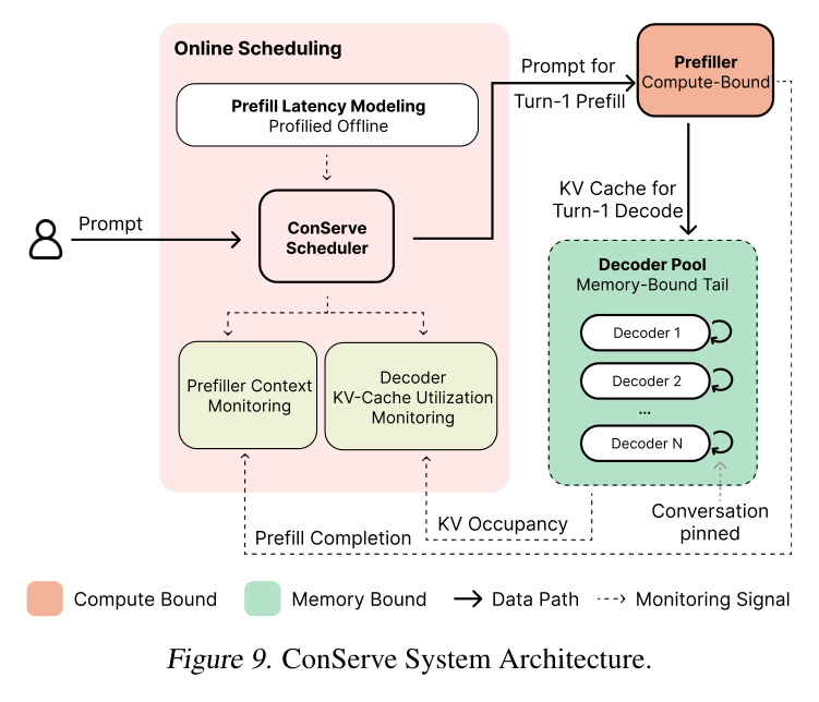
Paper's Figure 9 (caption: "ConServe System Architecture"). The system runs PD-disaggregated: one prefiller node processes input prompts, N decoder replicas generate output. A conversation is bound to one decoder at arrival and stays there for life; turn-1 prefill runs on the prefiller, its KV cache transfers once to the bound decoder, and all later turns' incremental prefill + decode run locally on that decoder with full KV reuse. One routing decision per conversation, zero decode-side prediction.

The per-turn agent loop and how ConServe places it:

• Memory model: short-term = the growing KV cache pinned on the bound decoder (never re-transferred); long-term/episodic memory is external to ConServe (agent-side).
• Tool invocation: ReAct — structured tool call, suspend, resume with result appended; from ConServe's view a tool call is a wall-clock gap (W includes it) during which the KV slot stays reserved.
• Error recovery: ConServe never migrates an already-placed conversation. Under prefiller saturation or decoder KV pressure, it routes the next conversation elsewhere rather than reshuffling live ones — so a placement is never revisited.

Planning & reasoning #

• Planning style: not a reasoning agent per se — ConServe is a reactive scheduler. Placement is a fixed policy conditioned on observable state, deliberately not a search or learned planner.
• Decomposition: top-down — the conversation is decomposed once into (compute-bound prefill phase, memory-bound tail phase).
• Budget: provisioning is bounded by two decoder-side constraints (throughput and memory, §4) and one prefill saturation point $R^{*}$; there is no per-turn token/step budget.
• Backtracking: none by design — the "commit once, never revisit" property is what removes prediction from the loop.

4. 作者证明 #

This is an analytical-provisioning model, not a formal-guarantee proof: 无形式化作者证明 — 仅实证 for the scheduling outcome (latency/SLO/energy). What could have been bounded but is left empirical: end-to-end TTFET as a function of arrival rate, and the SLO-violation rate under prediction error. The paper does give a closed-form provisioning model for how many decoders to allocate.

Notation table

方程物理意义. Two decoder-side constraints must hold simultaneously:

$$N \cdot T_{d} \geq R \cdot L_{d} \quad \text{(throughput)}$$

$$N \cdot B \geq R \cdot W \quad \text{(memory)}$$

Constraint 1: aggregate decoder throughput must keep up with total token demand. Constraint 2: aggregate KV slots must hold every concurrently-live conversation, including those blocked on tool calls. The prefill node saturates at

$$R^{*} = \frac{T_{p}}{L_{in}}$$

ConServe picks integer $N$ that over-satisfies both inequalities at $R = R^{*}$, deliberately placing the bottleneck on the prefiller — where the driving signal (input token rate) is observable at admission and maps deterministically to utilization via the offline latency curve.

Six minimum checks:

1. Units. Eq.1: $[N][T_d]$ = (replicas · tokens/s/replica) = tokens/s; RHS $[R][L_d]$ = (conv/s · tokens/conv) = tokens/s. ✓ balanced. Eq.2: $[N][B]$ = slots; $[R][W]$ = (conv/s · s) = conversations. ✓.
2. Limiting case $R \to 0$. Both RHS → 0, so any $N \geq 1$ satisfies; matches intuition (idle system needs one replica).
3. Limiting case $L_{in}$ large. $R^{*} = T_p/L_{in} \to 0$: very long turn-1 prompts saturate the prefiller at a low arrival rate — consistent with the quadratic prefill regime (Fig.2).
4. Monotonicity. $N$ required grows linearly in $R$ under both constraints; increasing $T_d$ or $B$ lowers required $N$. Consistent.
5. Sanity number. With 15k in + 1k out per conversation the paper computes ≥1.67 decoders/prefiller; they deploy 3, i.e. over-provisioned so the prefiller saturates first. ✓ internally consistent.
6. Binding constraint. Which of Eq.1/Eq.2 binds depends on the input/output ratio; the design chooses $N$ so that neither decoder constraint binds before $R^{*}$, i.e. the prefiller is always the first bottleneck. ✓ matches the "bounded prefiller load" SLO argument (§5.3).

Agent-specific asks #

• Success-rate / sweep model: the paper sweeps arrival rate (0.5→1.634 conv/s) × system (5 baselines) × wrong-prediction rate (0→50% for AMPD) × hardware (homogeneous vs 200W-capped). Monotonicity holds: latency and SLO violations grow ~linearly in AMPD's error rate; ConServe is flat along that axis by construction.
• Latency budget per turn: prefiller ~25k input tok/s; each decoder ~1k output tok/s and ~300k KV tokens; KV transfer happens once per conversation and is dominated by quadratic prefill at agentic input sizes (Fig.3). The paper does not claim a hard "interactive latency" bound but demonstrates zero SLO violation at the 5× threshold.
• Failure-mode classification: three failure classes for the per-turn baseline (§5.4) — (i) cost model ignores decoder KV utilization, (ii) collocation-batch variance uncapturable offline, (iii, dominant) prefiller queueing pressure from misrouted turn-2+ prefills. ConServe's design targets exactly (iii) by never routing turn-2+ to the prefiller.

5. 实验与数据 #

Workload: SWE-bench_bm25_13K traces via swe-agent (generated with Qwen3-Coder-30B-A3B), replayed on a 4-GPU A40 machine serving Qwen3-0.6B (small served model chosen for KV headroom). Baselines: Collocated, Full Disaggregation, AMPD (per-turn prediction).



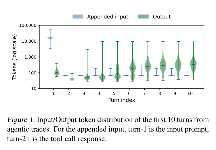
Paper's Figure 1. Turn-1 input is tens of thousands of tokens; turn-2+ appends (tool responses) are hundreds. Output-token counts are high-variance and unpredictable — the empirical root of why decode-side cost cannot be forecast, motivating the whole thesis.



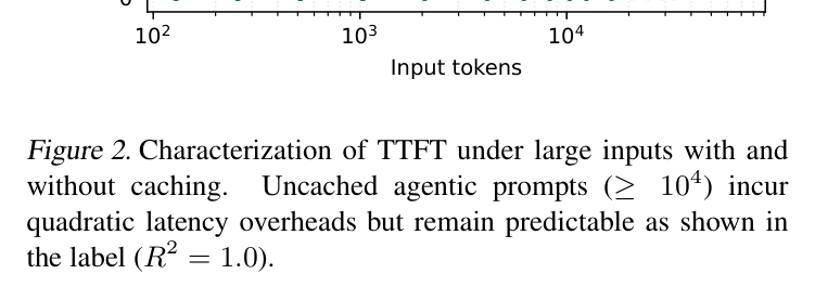
Paper's Figure 2 (caption notes $R^2=1.0$). Uncached prefill TTFT grows quadratically (attention-dominated) once inputs exceed $10^4$ tokens — contradicting the common linear model — but is highly predictable ($R^2=1.0$). Prefix caching flattens TTFT to near-constant, cutting latency ~2 orders of magnitude at long inputs. This is what makes turn-1 input length a usable deterministic scheduling signal.



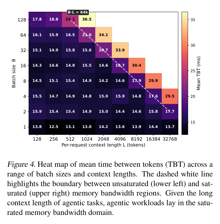
Paper's Figure 4. Mean TBT is stable at small batch/context but climbs sharply once memory bandwidth saturates (upper-right of the dashed boundary). Agentic tasks' long contexts sit firmly in the saturated (memory-bound) region — confirming the tail phase is memory-bound.



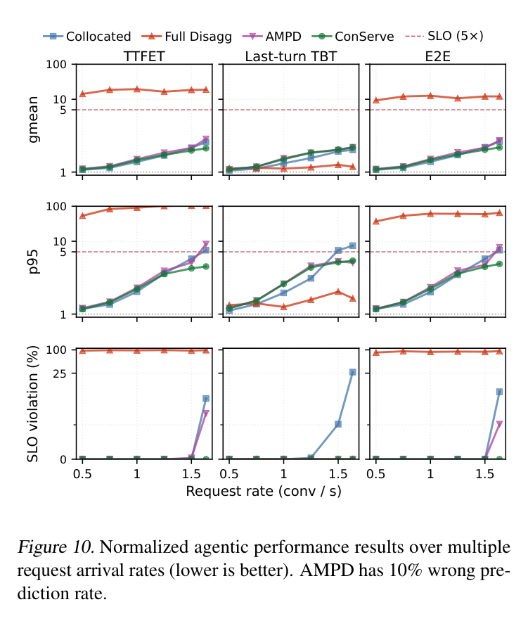
Paper's Figure 10 (AMPD at 10% wrong prediction). The load-bearing result: at saturation ConServe holds steady on p95 TTFET while Collocated and AMPD degrade sharply. Full Disaggregation is >10× baseline on TTFET/E2E (it re-pays prefill + KV transfer every turn) yet wins last-turn TBT (1.35× vs ConServe's 2.49×) — a baseline that dominates one metric while losing the headline one.



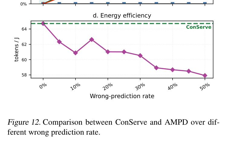
Paper's Figure 12. At 0% error AMPD reduces exactly to ConServe (local turn-2+ execution always dominates in this workload), so the per-turn mechanism only ever adds error, never benefit. At 5% error, SLO violations already reach ~7.8% (TTFET)/6.3% (E2E); by 50% both grow linearly past 50% violations and tokens-per-joule declines toward 58 tok/J. This linear degradation is the paper's core empirical demonstration of structural brittleness; ConServe has no such curve.

6. 论证链 #

#	Step	Support
1	Agentic conversations = one long compute-bound turn-1 prefill + a long memory-bound tail of short appends (input distribution).	§1, §3 / Fig.1
2	Turn-1 prefill TTFT is a deterministic (quadratic, $R^2=1.0$) function of input length; prefix caching makes turn-2+ prefill near-free; KV transfer is marginal at agentic input sizes.	§3.1 / Fig.2, Fig.3
3	Decode is memory-bound and its per-iteration/end-to-end latency is high-variance and unpredictable.	§3.2 / Fig.4, Fig.5, Fig.6
4	Therefore per-turn schedulers must predict unobservable decode-side cost; raising the unit to the conversation makes placement depend only on observable turn-1 input length + KV occupancy.	§1, §4.2
5	Provisioning $N$ decoders to over-satisfy the throughput/memory constraints at $R^{*}$ places the bottleneck on the observable prefiller, bounding its load → zero SLO violations by construction.	§4.1, §5.3 / Fig.10
6	Per-turn prediction degrades SLO/energy linearly with error rate; ConServe stays flat.	§5.4 / Fig.12
7	The compute/memory phase split maps onto GPU tiers: capping decoders to 200W adds +22.75% tokens/J with unchanged latency, since the memory-bound tail absorbs the power cut.	§3.3, §4.3, §5.5 / Fig.7, Fig.8, Fig.13

7. 实现 cross-reference #

Built on vLLM (Kwon et al. 2023) as the serving engine and LMCache (Cheng et al. 2025) as the PD-disaggregation manager. No public ConServe repository is referenced in the source. [实现未公开]

核心技术壁垒 (single hardest-to-replicate insight). The value is not an engineering trick but the reframing: recognizing that prediction dependence is imposed by the scheduling unit, not the workload, and that coarsening to the conversation collapses turn irregularity into the classical two-phase (compute-bound / memory-bound) abstraction with a single KV-transfer boundary. Everything else (reactive placement, over-provisioning, tier mapping) follows mechanically once you accept the conversation is the unit. Replicating the idea is trivial; arriving at it against the field's per-turn default is the hard part, and it is validated by the fact that the strongest per-turn baseline degenerates to ConServe at 0% error (its mechanism is net-negative here).

关键实现细节 (easy-to-miss tricks).

1. Deliberate prefiller-first bottleneck. $N$ is over-provisioned (3 decoders when ≥1.67 suffice) specifically so the prefiller — whose load is the only observable, deterministic signal — saturates before the decoders. This is what converts "SLO robustness" from a tuning outcome into a structural guarantee.
2. Pin-and-never-migrate + bind to lowest-KV-occupancy decoder. After the one KV transfer, the conversation is pinned; new conversations bind to the decoder with lowest current KV occupancy, and saturation is handled by routing the next conversation elsewhere rather than migrating a live one. This keeps KV state from ever crossing the network more than once and removes any per-turn re-evaluation.

Tool & environment interface #

• Tool catalog: opaque to ConServe — tool calls are the agent's; the scheduler only sees the resulting wall-clock suspension and appended short input.
• Side effects: the KV cache is the only state ConServe mutates; it decrements occupancy on conversation termination so the signal reflects active (not allocated-but-idle) memory.
• Error surface: a saturated prefiller / KV-pressured decoder surfaces as an observable state, not an exception — capacity management uses the same two signals as placement.
• Environment contract: decoder is assumed to hold KV across turns (stateful within a conversation) and tool-call time is folded into lifetime $W$.

LLM backbone requirements #

• Served model here is Qwen3-0.6B — deliberately tiny to leave KV-cache headroom, not a capability floor for the method (the scheduler is model-agnostic). Traces were generated by a much larger Qwen3-Coder-30B-A3B, so decode dynamics reflect a 0.6B backbone while the trajectory shape comes from the 30B agent.
• Required capability: ReAct-style tool-call formatting; long-context prefill.
• Sensitivity: qualitative observations claimed to hold across model sizes/GPU generations since they are architectural (compute-bound prefill / memory-bound decode) rather than config-specific.

Evaluation #

• Benchmark: SWE-bench (bm25_13K) traces with swe-agent. Metrics: TTFET (new, conversation-level), last-turn TBT, E2E latency; plus conventional per-turn TTFT/TBT CDFs for comparison. SLO = 5× single-request baseline latency per metric.
• Baselines: Collocated, Full Disaggregation, AMPD (He et al. 2026, per-turn prediction; PPD by Li et al. 2026 discussed but AMPD is the implemented primary baseline).
• Caveat: AMPD's bidirectional KV transfer was simulated (latency modeled, traces post-processed), not fully re-implemented.

Production readiness #

• Sandboxing / secrets: out of scope — the paper serves inference, not tool execution.
• Observability: placement is deterministic from two logged signals (input length, KV occupancy), so scheduling decisions are reproducible even though decode itself is non-deterministic.
• Cost / concurrency controls: over-provisioned decoders absorb length variation; autoscaling triggers off the same observable prefiller-saturation and KV-pressure signals — no learned cost model to retrain.