Maestro: Workload-Aware Cross-Cluster Scheduling for LLM-Based Multi-Agent Systems
Maestro: Workload-Aware Cross-Cluster Scheduling for LLM-Based Multi-Agent Systems #
1. TL;DR #
Serving LLM multi-agent workflows under tight GPU budgets breaks because each stage's decode length and KV footprint are unknown, model demand is long-tailed, and clusters differ in readiness vs latency. Maestro predicts per-stage output length and KV need (tool-intent classifier + role-aware regressor), then drives node-level hierarchical weight residency + elastic KV, cross-cluster fitness routing, and boundary-preemptive SRTF. Result: −67.2% KV-reservation HBM, +23.6 pp SLO over EDF.
2. Q1 / Q2 / Q3 #
Q1 — 痛点. LLM-MAS treats one user query as a dependency-coupled workflow of stages (e.g. Planner → Coder → Reviewer), each an LLM call whose latency and memory scale with an unknown-in-advance output length. Three concrete failures follow: (a) non-deterministic per-stage cost causes head-of-line (HoL) blocking where a long reasoning step delays short interactive ones; (b) model invocation is heavy-tailed — a few models are hot, most are cold — so dedicating a GPU per model wastes capacity while on-demand loading incurs tens-of-seconds cold starts that break interactive SLOs; (c) in a multi-cluster setting the nearest cluster (low RTT) may lack the warm model or KV headroom, while a farther cluster is ready. Existing systems either target single-turn queries with fixed partitioning (FastServe, MuxServe, QLM) or do static cross-cluster routing oblivious to model readiness (SkyServe, AIBrix). None couples stage-level cost estimation with cross-cluster allocation for agentic workflows.
Q2 — 方法. Maestro characterizes each workflow stage along five agent-level dimensions (role/position, tool-invocation intent, predicted output length + KV footprint, remaining workflow time, per-cluster model readiness) and coordinates three tiers in one closed loop: node-level memory-safe multi-model colocation via GPU→CPU→disk hierarchical residency + prediction-guided elastic KV; cluster-level fitness-based dispatch balancing RTT, model readiness, and KV feasibility; global-level workflow-aware preemptive SRTF that protects latency-critical stages without starving long jobs. The forecasting stack is a two-stage predictor: an isotonic-calibrated LightGBM tool-intent classifier feeds a role-specific length regressor trained on $\log(1+L)$ to tame the heavy tail.
核心技术壁垒: the load-bearing insight is that tool-invocation intent is a first-class, cheaply-predictable signal that splits the bimodal output-length distribution — modeling it explicitly (stage-1 classifier as a continuous calibrated feature into stage-2 regression) is what makes stage cost estimable enough to drive SRTF, KV admission, and routing simultaneously. Everything downstream (Eqs 2, 3, 5, 7) consumes $\hat{L}$ / $\hat{p}_{\mathrm{tool}}$; without a low-error length estimate the whole three-tier loop degrades to blind heuristics. Detailed in §7.
Q3 — 结果. On a 32-server A100 testbed + trace-driven simulation (46,769 jobs / 144,524 stages across 9 apps): length-prediction MAE cut 19.2% vs Magnus; KV-reservation HBM cut 67.2% (205% overcommit, 3.05× effective footprint on a 40 GB GPU); high-contention SLO attainment +23.6 pp over EDF (50.0% → 73.6% at $\lambda=2.0$, batch=0.8) with −84.8% interactive queueing delay.
3. 架构 / 方法图 #
Maestro's system architecture and end-to-end workflow:
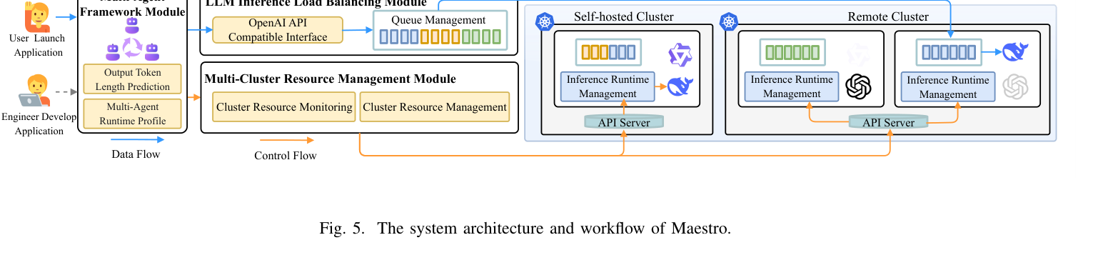
Paper's Figure 5 ("The system architecture and workflow of Maestro"). The figure shows the stage-driven closed loop: an incoming workflow stage is intercepted at the dispatch gateway, described (role/position/tool availability + semantic embedding), cost-predicted, then routed by the global scheduler to a node whose runtime manages hierarchical weight residency and elastic KV; post-execution telemetry recalibrates the predictor. Readers should notice that scheduling, node memory management, and prediction are not separate services but signal-coupled stages of one control loop.
The two-stage cost predictor architecture:
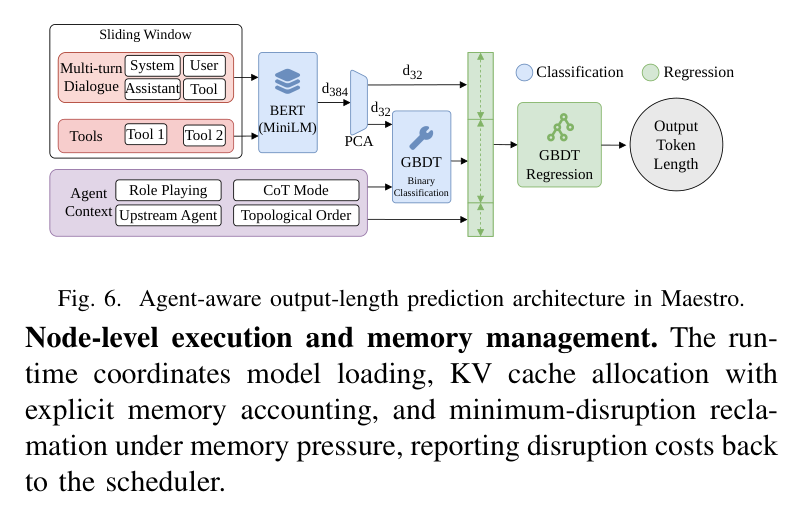
Paper's Figure 6 ("Agent-aware output-length prediction architecture in Maestro"). Structured features (role, workflow position, invocation index, tool availability) are concatenated with a sliding-window MiniLM semantic embedding; a first-stage tool-intent classifier emits a calibrated probability that is fed as a continuous feature into the second-stage length regressor. The key structural point is the explicit intermediate tool-intent node — it is the mechanism that separates the short-structured vs long-free-form output modes.
The per-turn agent scheduling loop, redrawn as a state machine for the five-phase pipeline that the raster figure narrates in prose:
The recovery edge matters: when node-level KV admission fails, the runtime does not silently OOM — it computes a minimum-impact degradation plan and reports the disruption cost back, so the scheduler can fall back to re-routing or re-queueing at a stage boundary.
Agent scope. Task class: open-ended agentic workflows (interactive assistants + batch analytic pipelines) covering serial, parallel, loop, and supervisor-worker topologies. Interaction pattern: multi-turn dependency-coupled stages per job. Autonomy: fully autonomous execution; the system under study is the serving/scheduling substrate, not the agent policy. Memory model here is systems-level (KV cache = short-term working state, hierarchical weight tiers = long-term residency), not an agent-cognition memory. Planning style is a predetermined workflow template (not ReAct/ToT search); Maestro exploits the template's rolling execution profile (Eq. 8) rather than performing task planning itself. Budgeting is expressed as GPU-memory feasibility + remaining-time estimates rather than max-step counts.
4. 作者证明 #
无形式化作者证明 — 仅实证. Maestro provides no convergence/optimality proof; it is an empirical systems paper. What could have been bounded but was not: SLO attainment as a function of prediction error $\rho$, or a competitive-ratio bound for the SRTF approximation against Oracle-SRTF. The paper instead relies on a cost model plus sweeps. Notation and the load-bearing equations:
| Symbol | Meaning |
|---|---|
| $T_{\mathrm{TTLT}}$ | time-to-last-token of a stage |
| $P,\ L,\ \hat{L}(T)$ | prompt length, true / predicted output length |
| $t_{\mathrm{dec}}(M)$ | avg per-token decode latency on model $M$ |
| $\hat{p}_{\mathrm{tool}}(T)$ | predicted tool-invocation probability |
| $\hat{R}_{\mathrm{kv}}(T),\ \alpha(M)$ | predicted KV need; per-token per-model memory coeff |
| $M_{\mathrm{res}},\ M_{\mathrm{kv}},\ M_{\mathrm{total}}$ | reserved non-KV footprint, current KV usage, total GPU mem |
| $R_{\mathrm{kv}}^{\mathrm{head}}(N)$ | KV admission headroom on node $N$ |
| $C_{\mathrm{deg}}(N,T)$ | disruption penalty of a degradation plan |
| $S(N,T),\ T_{\mathrm{ready}},\ T_{\mathrm{act}}$ | node fitness score, time-to-start, activation latency |
| $R_{\mathrm{need}}(T),\ \rho$ | safety-margined KV demand, EWMA-driven margin |
| $\widehat{T}_{\mathrm{rem}}(J,k)$ | estimated remaining workflow time (SRTF key) |
Cost model (motivates length prediction): $T_{\mathrm{TTLT}}=T_{\mathrm{prefill}}(P)+L\cdot t_{\mathrm{decode}}$ — for large $L$ the decode term dominates, so underestimating $L$ underestimates runtime. Predicted execution time reuses this additive form with calibrated microbenchmarks: $\widehat{T}_{\mathrm{exec}}(T)=t_{\mathrm{pre}}(P(T),M(T))+t_{\mathrm{dec}}(M(T))\cdot\hat{L}(T)$. KV scales linearly: $\hat{R}_{\mathrm{kv}}(T)=\alpha(M(T))\cdot(P(T)+\hat{L}(T))$. Node safety: $M_{\mathrm{kv}}+M_{\mathrm{res}}\leq M_{\mathrm{total}}$ with headroom $R_{\mathrm{kv}}^{\mathrm{head}}(N)=M_{\mathrm{total}}-M_{\mathrm{res}}-M_{\mathrm{kv}}$. Routing score $S(N,T)=A(N,T)-\lambda\,T_{\mathrm{ready}}(N,T)-\mu\,C_{\mathrm{deg}}(N,T)$ where $T_{\mathrm{ready}}=T_{\mathrm{q}}+T_{\mathrm{act}}$ and $T_{\mathrm{act}}\approx\text{Size}/\mathrm{BW}_{\mathrm{tier}}$. SRTF key $\widehat{T}_{\mathrm{rem}}(J,k)=\widehat{T}_{\mathrm{exec}}(T_k)+\widehat{T}_{\mathrm{future}}(J,k)$ with $\widehat{T}_{\mathrm{future}}(J,k)\approx T^{(0.50)}_{\mathrm{next}}(\mathrm{state}(J,k))$.
Six minimum checks:
- Success-rate sweep. SLO attainment is swept over arrival rate $\lambda\in[0.4,2.0]$ and batch ratio $[0.20,0.80]$ (Fig 7); it is monotone-decreasing in load and batch ratio for all methods, and Maestro's advantage over EDF widens under contention (peak +23.6 pp). Reproducible: fixed templates, distinct prompts train/test.
- Latency budget per turn. Prediction adds median 11.24 ms (Fig 9) — negligible vs inter-region RTT (tens–hundreds of ms) and cold-start (tens of s). The paper's interactivity claim rests on this ordering; verified by the overhead measurement.
- Failure-mode classification. Node-level failure is handled by five degradation levels (Idle→Sleeping, evict Sleeping, stop pending sleeps, swap KV of Active, abort Active) with ascending cost; the method targets the dominant class (KV admission failure under colocation) via minimum-impact greedy planning (Alg 2).
- Ablation monotonicity. Removing tool-intent classifier (w/o C) and then semantic embeddings (w/o BERT) monotonically worsens $R^2$ (0.7774 → 0.7722 → 0.7129), confirming each component's marginal contribution (Table VII).
- Baseline loss rows. Maestro is not free: vs exclusive deployment it is +3.0% (2 GPU) / +12.1% (1 GPU) slower (Table IV); MLP_BayesOpt_3 edges it on F1/Acc (0.9022 vs 0.8999, Table III) — accepted because Maestro wins on calibration (log loss), the property that matters for feeding the regressor.
- Upper-bound sanity. Oracle-SRTF (perfect remaining-time) is included as an explicit upper bound; Maestro's approximation via Eqs 7–8 is measured against it under the same vLLM backend and arrivals.
- Regress on $\log(1+L)$, invert at inference — without the log transform the heavy tail dominates the loss and $R^2$ collapses (Linear baseline hits negative $R^2$). This one preprocessing choice is load-bearing for the accuracy claim.
- Sleeping state ≠ free — offloading weights to host but retaining CUDA graphs / JIT kernels costs 194–286 MB/model of GPU context (Table V), explicitly booked into $M_{\mathrm{res}}$ and traded against activation latency; a re-implementation that forgets this context footprint will over-report achievable overcommit. Boundary-only preemption (between LLM invocations, with hysteresis + EWMA smoothing + aging) is the other quiet correctness detail that avoids oscillation and starvation.
5. 实验与数据 #
Motivation measurements. Output length is bimodal and role/mode-dependent:

Paper's Figure 1 ("Output-token length distributions under non-CoT and CoT settings, tool-call and non-tool-call"). Tool-call stages cluster at short lengths; CoT and non-tool stages have a heavy tail. This bimodality is the empirical justification for the two-stage predictor — a single regressor would average across the two modes.
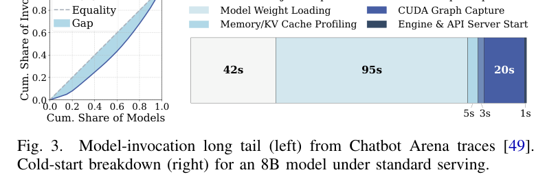
Paper's Figure 3 (left: model-invocation long tail from Chatbot Arena traces; right: cold-start breakdown for an 8B model). The long tail (few hot models, many cold) is why per-model GPU dedication wastes capacity, and the cold-start breakdown (tens of seconds) is why naive on-demand loading violates interactive SLOs — jointly motivating hierarchical residency + the Sleeping state.
Overall scheduling result — the headline SLO/latency evidence:
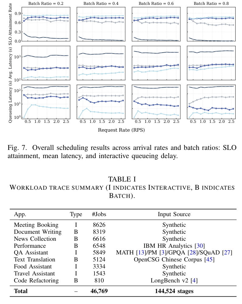
Paper's Figure 7 ("Overall scheduling results across arrival rates and batch ratios: SLO attainment, mean latency, and interactive queueing delay"). FCFS collapses (<10% SLO) under HoL blocking; EDF is better but degrades as long jobs near deadlines; Maestro holds 73.6% vs EDF 50.0% at the stress point and cuts interactive queueing delay 84.8%. This is the load-bearing figure for the "+23.6 pp over EDF" claim.
Memory overcommitment (source of the 67.2% number), Table V — five Qwen3 models colocated on a single 40 GB A100:
| Model | CUDA Graph | Weight Size | Virtual KV Cache |
|---|---|---|---|
| Qwen3-0.6B | 194 MB | 1.12 GB | 34.24 GB |
| Qwen3-1.7B | 194 MB | 3.21 GB | 32.15 GB |
| Qwen3-4B | 256 MB | 7.55 GB | 27.81 GB |
| Qwen3-8B | 245 MB | 15.27 GB | 20.07 GB |
| Qwen3-14B | 286 MB | 27.52 GB | 7.74 GB |
Total virtual KV ≈122 GB on a 40 GB GPU = 3.05× effective footprint (205% overcommit, 67.2% less HBM than non-overcommitted reservation); preserved contexts cost 194–286 MB/model (~1.15 GB total), explicitly counted in $M_{\mathrm{res}}$.
Utilization under colocation:
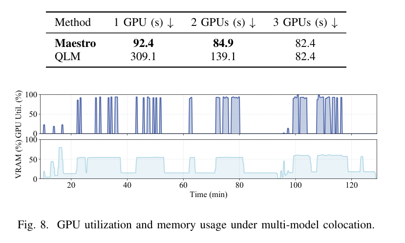
Paper's Figure 8 ("GPU utilization and memory usage under multi-model colocation"). Utilization is highly intermittent under low load, showing exclusive deployment would waste capacity; Maestro keeps models warm and overcommits memory safely — the visual case for spatial+temporal multiplexing.
Cost–latency case study (Table IV, Travel Assistant, 6 invocations / 3 models):
| Method | 1 GPU (s) ↓ | 2 GPUs (s) ↓ | 3 GPUs (s) ↓ |
|---|---|---|---|
| Maestro | 92.4 | 84.9 | 82.4 |
| QLM | 309.1 | 139.1 | 82.4 |
Maestro cuts completion time 38.9% (2 GPU) and 70.0% (1 GPU) vs QLM's process-restart switching; strikingly, Maestro at 1 GPU (92.4 s) beats QLM at 2 GPUs (139.1 s).
Prediction accuracy (Table VI) and preemption ablation (Table II):
| Metric | Maestro-Pred | Magnus | BERT-MLP | Linear |
|---|---|---|---|---|
| MAE ↓ | 165.43 | 204.74 | 239.33 | 496.86 |
| $R^{2}$ ↑ | 0.7774 | 0.6721 | 0.5620 | -0.3177 |
Linear's negative $R^2$ confirms output length is not a simple function of input length. Under extreme load ($\lambda=5.0$, batch=0.6), preemption raises SLO 60% vs 27% (2 nodes) and 75% vs 59% (4 nodes), and cuts delay to 2 ms vs 11 s (5 nodes) — though SLO is non-monotonic in node count (29%→60%→38%→75%→85%), an unexplained 3-node dip.
6. 论证链 #
| # | Step | Support (paper-internal) |
|---|---|---|
| 1 | Stage latency & KV both scale with output length $L$, which is unknown a priori. | Cost model $T_{\mathrm{TTLT}}=T_{\mathrm{prefill}}(P)+L\cdot t_{\mathrm{decode}}$; KV ∝ $(P+L)$ (§II). |
| 2 | Output length is bimodal, driven by tool-intent and CoT mode → predictable from agent features. | Observation-1, Fig 1/2; two-stage predictor cuts MAE 19.2% (Table VI). |
| 3 | With $\hat{L}$, $\hat{R}_{\mathrm{kv}}$ (Eqs 2–3), the node runtime can do explicit memory accounting and safely overcommit KV under $M_{\mathrm{kv}}+M_{\mathrm{res}}\leq M_{\mathrm{total}}$. | §III-C; Table V shows 205% overcommit / −67.2% HBM. |
| 4 | The same predictions feed a fitness score (Eq 5) that routes across clusters balancing RTT, readiness ($T_{\mathrm{act}}$), and disruption ($C_{\mathrm{deg}}$). | §III-D; Table VIII: bin-packing −58.3% queueing delay, affinity improves further. |
| 5 | Remaining-time estimates (Eqs 7–8) drive boundary-preemptive SRTF, curbing dependency-induced HoL blocking. | §III-D; Fig 7 (+23.6 pp SLO), Table II (preemption raises SLO, cuts delay orders of magnitude). |
7. 实现 cross-reference #
Implementation surface. Built on vLLM v0.11.0 (extending PagedAttention KV management with an elastic paging mechanism) integrating kvcached [ovg-projectKvcached2025] for CUDA VMM allocate/reclaim; deployed on Kubernetes v1.31.2, CUDA 13.0. Predictor uses MiniLM (sliding-window + mean-pool) for semantic features and LightGBM for both the tool-intent classifier and length regressor. The source paper does not release code; [实现未公开] for the scheduler/runtime source, but the three algorithms are fully specified as pseudocode in L1 (Alg 1 hierarchical residency, Alg 2 minimum-impact coordination, Alg 3 cross-cluster scheduling), so re-implementation is tractable.
核心技术壁垒 (the single hardest-to-replicate insight). The stage-1 tool-intent classifier as a calibrated continuous feature into stage-2 length regression. Its value is subtle: on raw accuracy a 3-layer MLP matches or beats it (F1 0.9022 vs 0.8999), but Maestro-Pred wins on log loss (0.2437, lowest) — and calibration, not accuracy, is what matters because the probability is consumed as a regression feature, not a hard label. Isotonic regression aligns predicted confidence with empirical frequency, and the fallback $\hat{p}_{\mathrm{tool}}=0$ when no tools exist keeps the signal well-defined. Getting this calibration right is the non-obvious step that makes the whole downstream loop (KV admission, SRTF, routing) trustworthy; a naively-trained classifier would inject miscalibrated noise into every scheduling decision.
关键实现细节 (easy-to-miss tricks).