LaWAM: Latent World Action Models for Efficient Dynamics-Aware Robot Policies — L2 #

§1 TL;DR #

LaWAM gives a VLA policy explicit dynamics foresight without generating future pixels: it keeps the forward decoder of a latent action model (usually thrown away) as a Latent World Model (LaWM) that expands a policy-predicted latent action into one latent visual subgoal in a single forward pass. Matches/beats pixel-space WAMs (98.6% LIBERO, 92.64 RoboTwin clean, 90.0 real-world) at 187 ms — up to 24× lower latency, 230M world-model params vs a 5B WAN backbone.

---

§2 Q1 / Q2 / Q3 #

Q1 — 痛点 (problem formulation) #

VLAs predict actions from the current visual-language context and never model how the scene changes under candidate actions. World-Action Models (WAMs) fix this by conditioning on predicted futures, but the dominant recipe — generate future images/video, then invert to actions — has three concrete costs:

1. Capacity misallocation: pixel synthesis burns modeling capacity on appearance-level detail that chunk-level control does not need.
2. Latency: iterative generation is slow. Under the paper's setup, LingBot-VA needs 4482 ms per inference vs 220 ms for the VLA $\pi_{0.5}$.
3. Wrong target: what control actually needs is the state change relevant to the next action chunk, not a visually plausible task-consistent future.

Formally, the WAM template factorizes the joint over (action chunk, horizon observation) as a future-prediction term times an inverse-dynamics term:

$$\underbrace{p(a_{1:T},o_{T}\mid o,l)}_{\text{Joint}}=\underbrace{p(o_{T}\mid o,l)}_{\text{Future Prediction}}\;\underbrace{p(a_{1:T}\mid o,o_{T})}_{\text{IDM}}.$$

The pain is that the "Future Prediction" term is instantiated in pixel space and rolled out iteratively.

Q2 — 方法 (method core) #

Represent the future in a frozen visual feature space instead of pixels. With a frozen encoder $f_\psi$, define $u=f_\psi(o)$ and $u_T=f_\psi(o_T)$. Stage 1 learns a latent action model over feature pairs — a posterior infers a latent action, and a decoder predicts the future feature:

$$z\sim q_{\phi}(z\mid u,u_{T}),\qquad \tilde{u}_{T}=\mathrm{LaWM}_{\omega}(u,z).$$

The 核心技术壁垒 is a single conceptual move: prior latent-action VLAs (LAPA, CoMo, Genie-style) use this decoder only as an auxiliary training crutch and discard it after pretraining, keeping only the latent-action space. LaWAM instead retains the decoder as the policy-facing dynamics interface — one non-iterative forward pass turns a policy-predicted latent action into a spatially structured latent visual subgoal. This is the hard-to-replicate insight: not a new loss or architecture, but recognizing that the LAM decoder already is a latent-action-conditioned world model, and building the whole inference path around it.

At test time $u_T$ is unavailable, so the policy must predict the latent action first. LaWAM factorizes inference into three terms — policy prior → deterministic LaWM decode → action expert:

$$\underbrace{p(a_{1:T},\hat{u}_{T},\hat{z}\mid o,l)}_{\text{LaWAM}}=\underbrace{p_{\theta}(\hat{z}\mid o,l)}_{\text{Policy Prior}}\;\underbrace{p_{\omega}(\hat{u}_{T}\mid u,\hat{z})}_{\text{LaWM}}\;\underbrace{p_{\eta}(a_{1:T}\mid o,l,u,\hat{u}_{T})}_{\text{Action Expert}}.$$

Before vs after the key mechanism:

	Prior latent-action VLA	LaWAM
LAM decoder	discarded after pretraining	retained as LaWM
Policy interface	raw latent action $z$	latent visual subgoal $\hat u_T=\mathrm{LaWM}(u,\hat z)$
Future prediction	none / pixel-space iterative	single-pass latent decode
Grounding	embodiment-agnostic token	current $u$ grounds $\hat u_T$ in this embodiment

Q3 — 结果 (results) #

• LIBERO: 98.6% average SR — best among VLA / latent-action / pixel-WAM baselines, at 187 ms and 2.3B params.
• RoboTwin 2.0: 92.64 clean average (best), 89.80 randomized (close to the strongest pixel-WAMs).
• Real-world: 90.0 average over 3 tasks, first on all three; especially decisive on towel folding where high-latency baselines act on stale cloth states.
• Efficiency: 230M LaWM replaces a 5B WAN backbone (~95% fewer world-modeling params); up to 24× lower wall-clock latency than pixel-space WAMs.

---

§3 架构 / 方法图 #



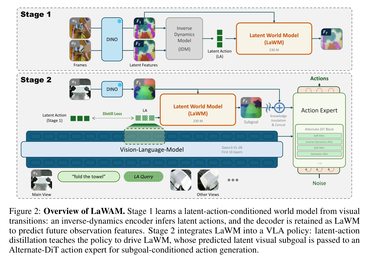
Paper's Figure 2, verbatim (caption: "Overview of LaWAM. Stage 1 learns a latent-action-conditioned world model from visual transitions: an inverse-dynamics encoder infers latent actions, and the decoder is retained as LaWM to predict future observation features. Stage 2 integrates LaWM into a VLA policy: latent-action distillation teaches the policy to drive LaWM, whose predicted latent visual subgoal is passed to an Alternate-DiT action expert for subgoal-conditioned action generation.").

This is the load-bearing architecture figure. Notice the asymmetry between stages: Stage 1's inverse-dynamics encoder consumes both current and future features to infer $z$ (only possible in training), while Stage 2 replaces that encoder with a policy prior that predicts $\hat z$ from the current observation alone — the decoder (LaWM) is shared and frozen across the two, which is exactly what makes the interface non-iterative at test time.

The data-path from a predicted subgoal to executed motion is best seen in the chunk-execution visualization:



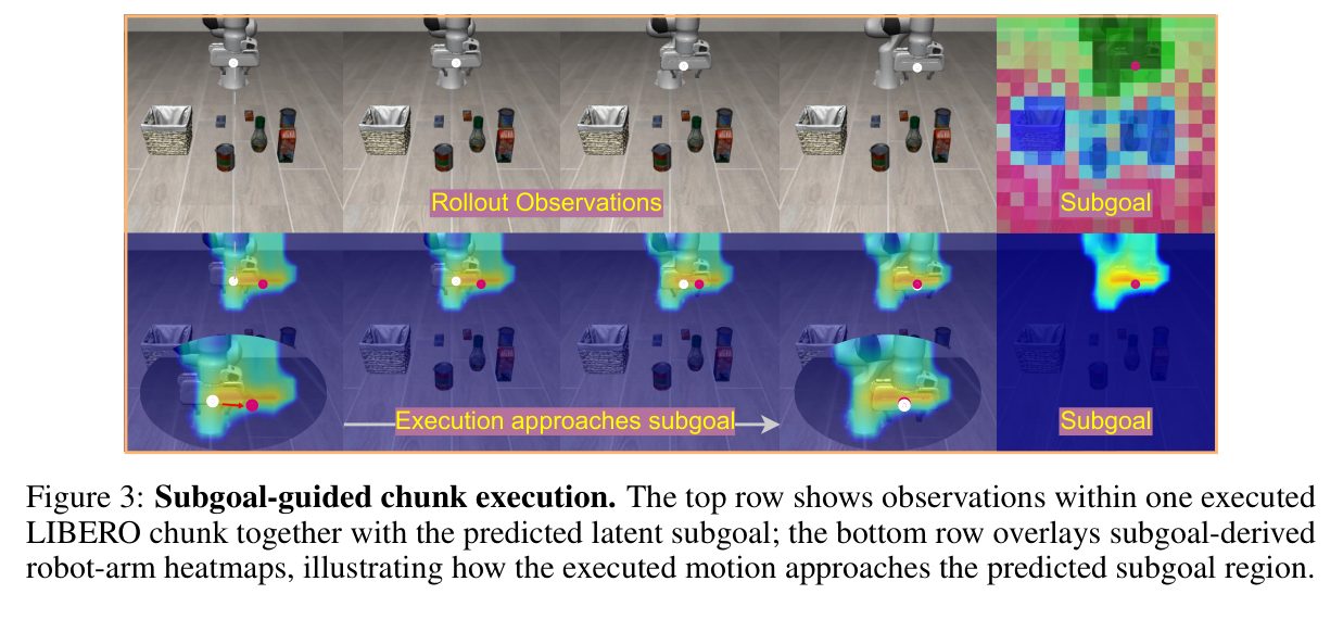
Paper's Figure 3, verbatim (caption: "Subgoal-guided chunk execution. The top row shows observations within one executed LIBERO chunk together with the predicted latent subgoal; the bottom row overlays subgoal-derived robot-arm heatmaps, illustrating how the executed motion approaches the predicted subgoal region.").

The heatmap overlay is a cosine-similarity map (a chosen robot-arm patch's DINO feature vs every patch in the predicted subgoal feature map). It makes the abstract "latent subgoal" concrete: the arm is expected to move toward the bright region, and the executed motion actually does — evidence the subgoal is action-relevant, not decorative.

---

§4 作者证明 #

无形式化作者证明 — 仅实证. LaWAM has no convergence theorem, variance bound, or proposition; its guarantees are entirely empirical. What it does provide is a set of well-motivated design equations, so the "proof" here is a notation + loss-decomposition audit rather than a theorem trace. A desirable formal result the paper lacks: a bound on subgoal prediction error $\lVert\hat u_T-u_T\rVert$ as a function of policy-prior latent-action error $\lVert\hat z-z\rVert$ (i.e. how faithfully the distilled prior can drive the frozen decoder), which would justify the distillation loss weight choice.

Notation table

Symbol	Meaning
$o,\;l$	current observation; task instruction
$a_{1:T}$	action chunk over fixed physical horizon $\tau$
$o_T$	horizon (future) observation after interval $\tau$
$f_\psi$	frozen visual encoder (distilled DINOv3 ViT-B/16)
$u=f_\psi(o),\;u_T=f_\psi(o_T)$	current / horizon latent features
$z\sim q_\phi(z\mid u,u_T)$	latent action; $q_\phi$ = latent inverse-dynamics posterior
$\mathrm{LaWM}_\omega(u,z)=\tilde u_T$	forward decoder = the retained world model
$\hat z,\;\hat u_T$	policy-predicted latent action; policy-driven subgoal
$p_\theta,\;p_\omega,\;p_\eta$	policy prior; LaWM decoder; action expert
$g(s,z)$	auxiliary state predictor; $s,s_T$ = EEF states
$\beta,\;\lambda_{\mathrm{distill}},\lambda_{\mathrm{wm}}$	KL weight ($10^{-5}$); loss weights ($0.1$)

Equation physical meaning. Stage-1 objective decomposes into three enforcers:

$$\mathcal{L}_{\mathrm{LAM}}=\mathcal{L}_{\mathrm{wm}}+\mathcal{L}_{\mathrm{aux}}+\beta\,D_{\mathrm{KL}}\!\left(q_{\phi}(z\mid u,u_{T})\,\|\,\mathcal{N}(0,I)\right).$$

• $\mathcal{L}_{\mathrm{wm}}=\lVert\tilde u_T-u_T\rVert_2^2$ forces the decoder to hit the true horizon feature (this is what makes it a world model).
• $\mathcal{L}_{\mathrm{aux}}=\lVert g(s,z)-s_T\rVert_2^2$ forces $z$ to carry embodied motion, not just visual appearance change.
• $\beta D_{\mathrm{KL}}$ shapes the latent-action space toward a Gaussian so the stage-2 policy prior can actually model it.

Stage-2 objective similarly decomposes:

$$\mathcal{L}_{\mathrm{LaWAM}}=\lambda_{\mathrm{distill}}\mathcal{L}_{\mathrm{distill}}+\lambda_{\mathrm{wm}}\mathcal{L}_{\mathrm{wm}}+\mathcal{L}_{\mathrm{act}}.$$

with $\mathcal{L}_{\mathrm{distill}}=\mathbb{E}[\lVert\hat z-z\rVert_2^2]$ (policy prior reproduces the teacher posterior's latent actions), $\mathcal{L}_{\mathrm{wm}}=\lVert\hat u_T-u_T\rVert_2^2$ (policy-driven subgoal stays near the true future), and $\mathcal{L}_{\mathrm{act}}$ the conditional flow-matching loss for the action chunk given $(o,l,u,\hat u_T)$.

6 minimum checks:

1. Dimensional/interpretive consistency — all three losses are squared-L2 in the DINO feature/state space plus a flow-matching term; units are consistent, no reward/log-prob mixing.
2. Assumption: fixed physical horizon $\tau$ — subgoal supervision assumes $u_T$ and $s_T$ come from the same elapsed time $\tau$ (not a frame offset). Breaks if datasets are mixed-frequency without correction — which is exactly why Eq. (6) $H_b=\mathrm{round}(\tau h_b)$ and Eq. (7) physical-time encoding exist.
3. Assumption: stable camera — the inverse-dynamics posterior assumes the transition $(u,u_T)$ is dominated by scene/embodiment change, not camera motion. The paper concedes (Limitations) that dominant camera motion collapses the latent-action space.
4. Determinism of decode — $p_\omega$ is used deterministically at inference ($\hat u_T=\mathrm{LaWM}_\omega(u,\hat z)$); the only stochasticity is the policy prior's $\hat z$ and the flow-matching sampler. Consistent with the "single forward pass" latency claim.
5. Teacher availability — distillation requires the stage-1 posterior $q_\phi$ as a frozen teacher; the encoder is kept solely to emit teacher $z$, never deployed. Self-consistent with the two-stage split.
6. KI necessity — Knowledge Insulation is claimed to stop action-expert gradients from overwriting LaWM dynamics; the ablation (§5) shows removing it degrades performance, supporting the claim that the frozen-teacher assumption in $\mathcal{L}_{\mathrm{distill}}$ genuinely needs gradient protection.

---

§5 实验与数据 #

LIBERO — the headline accuracy+efficiency claim.



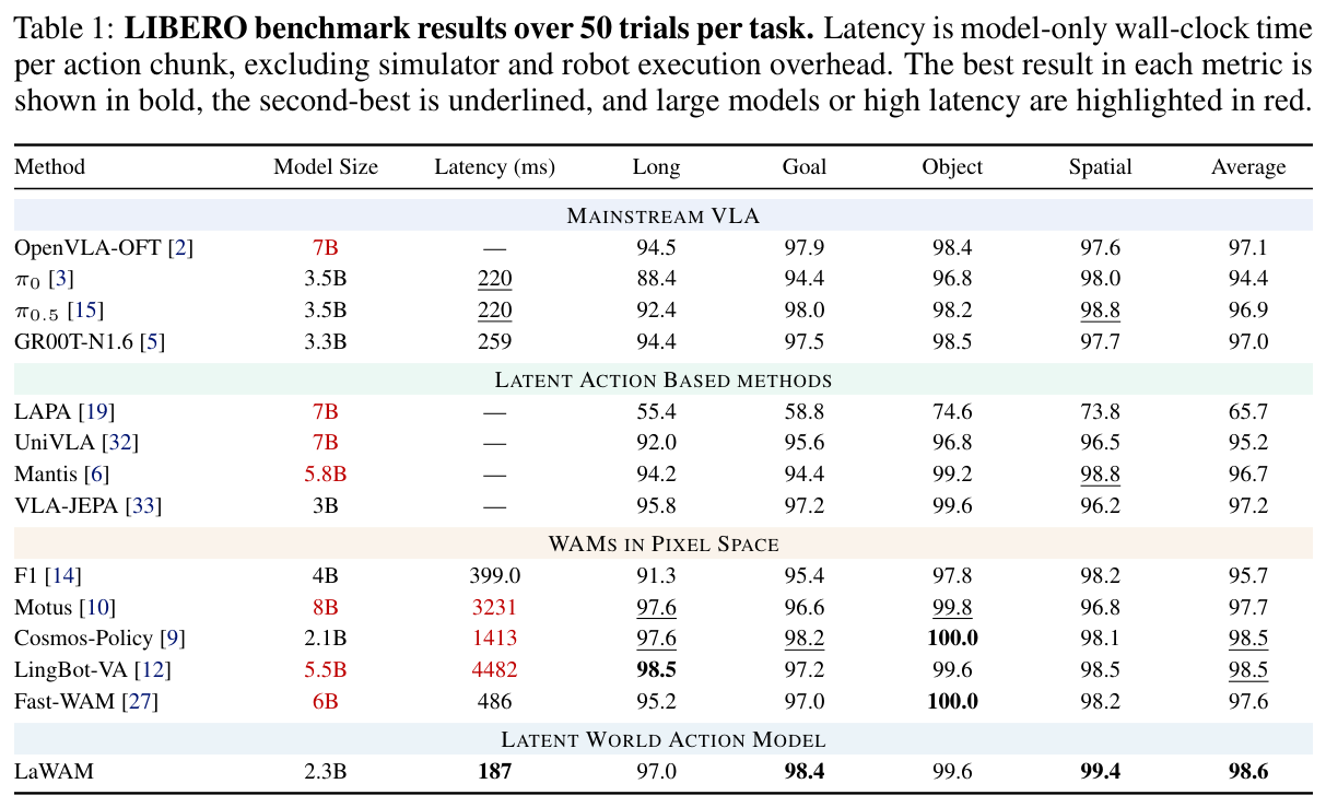
Paper's Table 1, verbatim (caption: "LIBERO benchmark results over 50 trials per task. Latency is model-only wall-clock time per action chunk... best in bold, second-best underlined, large models or high latency highlighted in red.").

The load-bearing comparison: LaWAM reaches 98.6 average at 2.3B / 187 ms, versus pixel-WAMs that match its accuracy only at 8–24× the latency (Motus 97.7 @ 3231 ms; LingBot-VA 98.5 @ 4482 ms; Cosmos-Policy 98.5 @ 1413 ms). Note LaWAM does not win every column — on LIBERO-Long it scores 97.0, below LingBot-VA's 98.5 — so the win is the accuracy/latency Pareto position, not a clean sweep.



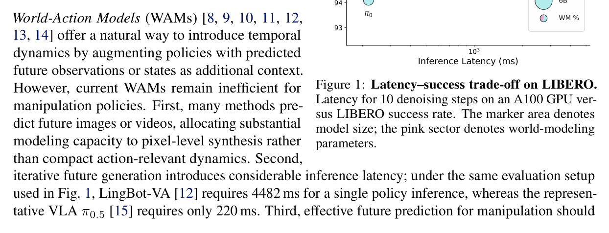
Paper's Figure 1, verbatim (caption: "Latency–success trade-off on LIBERO. Latency for 10 denoising steps on an A100 GPU versus LIBERO success rate. The marker area denotes model size; the pink sector denotes world-modeling parameters.").

This is the motivation-and-result figure in one: LaWAM sits at the top-left (high SR, low latency) with a small marker and a tiny pink world-modeling sector, while pixel-WAMs are pushed far right. The pink sector is the visual argument for the ~95% world-modeling parameter reduction.

RoboTwin — does it scale to bimanual?



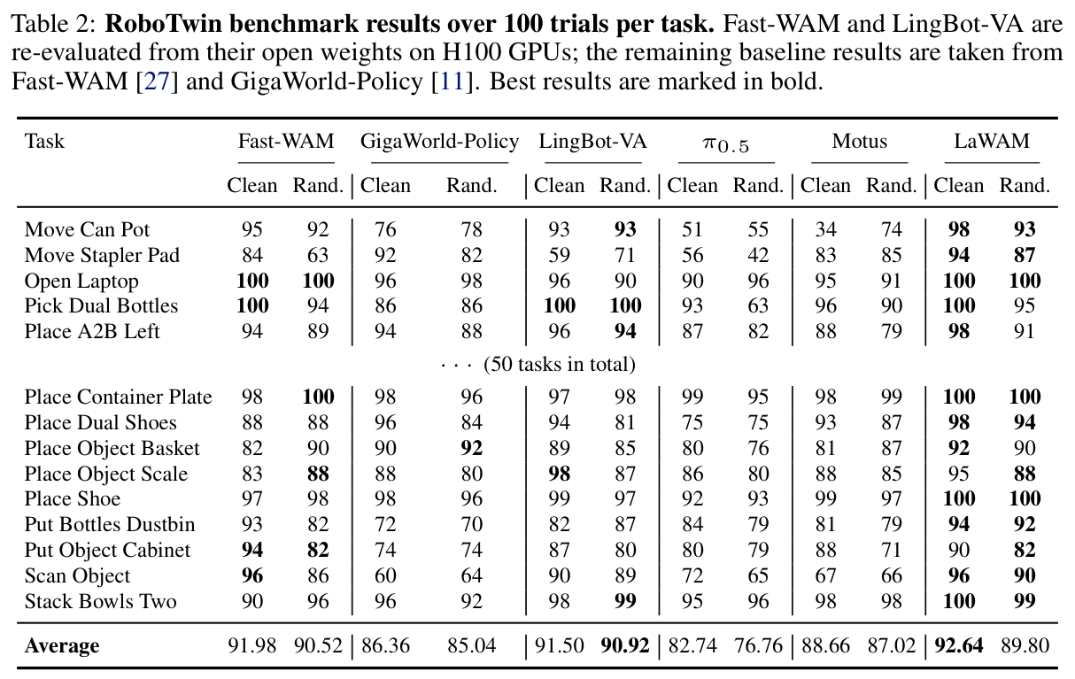
Paper's Table 2, verbatim (caption: "RoboTwin benchmark results over 100 trials per task... Fast-WAM and LingBot-VA re-evaluated from open weights on H100; remaining baselines from Fast-WAM and GigaWorld-Policy.").

LaWAM wins the clean-scene average (92.64) across 50 bimanual tasks, showing the latent-subgoal approach is not a single-arm LIBERO artifact. Honest caveat visible in the same table: on the randomized average (89.80) it trails Fast-WAM (90.52) and LingBot-VA (90.92), and it loses badly on a few tasks (Open Microwave, Turn Switch) — so robustness under heavy randomization is the current soft spot.

Ablation — which piece carries the gain?



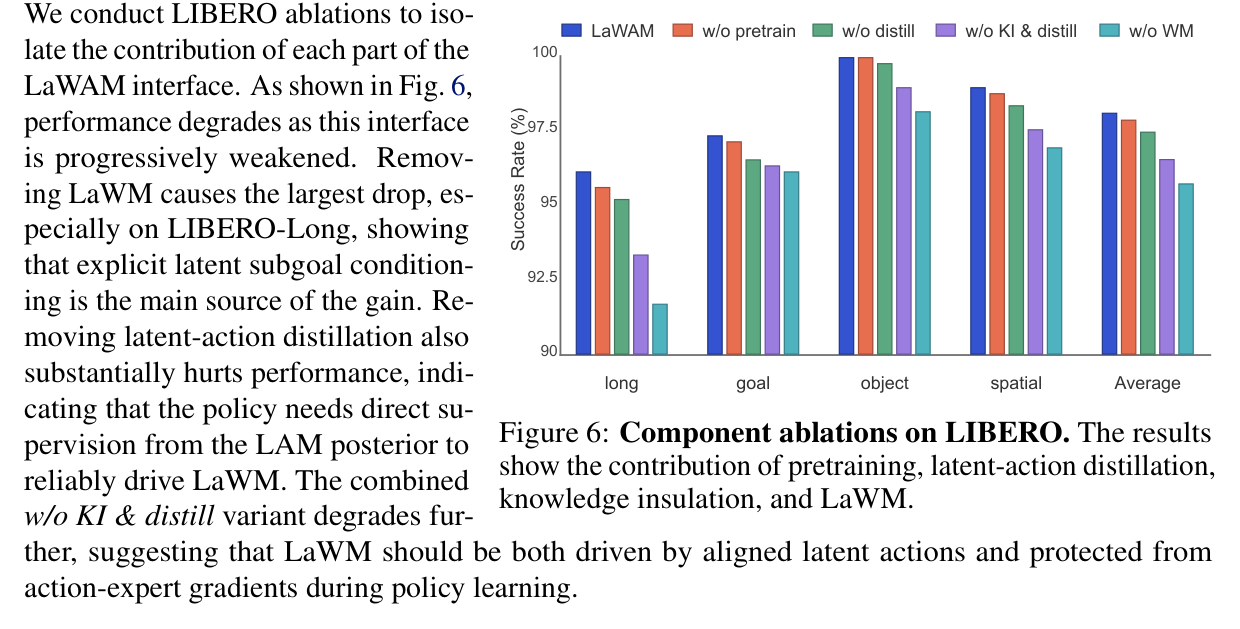
Paper's Figure 6, verbatim (caption: "Component ablations on LIBERO. The results show the contribution of pretraining, latent-action distillation, knowledge insulation, and LaWM.").

Removing LaWM causes the largest drop (especially on LIBERO-Long), directly validating that explicit latent-subgoal conditioning — not merely the latent-action tokens — is the main source of gain. Removing latent-action distillation is the second-biggest hit, showing the policy prior genuinely needs the LAM posterior's supervision to drive the decoder faithfully. The "w/o KI & distill" combined variant degrades further.

Does LaWM model real dynamics or just copy the input?



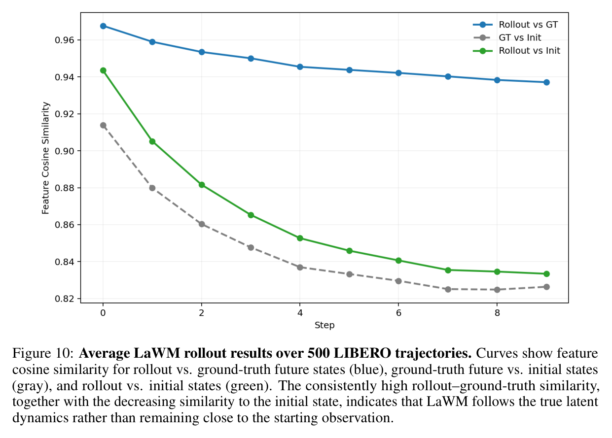
Paper's Figure 10, verbatim (caption: "Average LaWM rollout results over 500 LIBERO trajectories. Curves show feature cosine similarity for rollout vs. ground-truth future states (blue), ground-truth future vs. initial states (gray), and rollout vs. initial states (green).").

The blue curve (rollout vs GT future) stays high while the green curve (rollout vs initial) drops — quantitative evidence over 500 trajectories that LaWM follows true latent dynamics rather than trivially preserving the starting observation. This is the aggregate probe backing the qualitative subgoal heatmaps.

---

§6 论证链 #

Step	Claim	Paper-internal support
1	Pixel-space future generation is the bottleneck (capacity + latency + wrong target).	§1 three inefficiencies; LingBot-VA 4482 ms vs $\pi_{0.5}$ 220 ms; Fig. 1 / Table 1 latency column.
2	The future can be represented compactly in a frozen DINO feature space via a latent action model.	Eq. (2) feature-space LAM; §3.2 stage-1 training with $\mathcal{L}_{\mathrm{wm}}$ forward-prediction loss.
3	The LAM's forward decoder, if kept instead of discarded, is a usable non-iterative world model.	§2 (Garrido observation) + §3.2 "retain this decoder as LaWM"; single-pass $\hat u_T=\mathrm{LaWM}_\omega(u,\hat z)$.
4	A policy prior can be distilled to drive that decoder at test time (when $u_T$ is unavailable).	Eq. (3) inference factorization; Eq. (5) $\mathcal{L}_{\mathrm{distill}}$; §3.3 policy prior replaces IDM encoder.
5	Conditioning the action expert on the predicted subgoal via Alternate-DiT yields SOTA-competitive accuracy at far lower latency.	Table 1 (98.6 @ 187 ms), Table 2 (92.64 clean), Table 3 (90.0 real-world).
6	The subgoal conditioning (LaWM) — not the latent tokens alone — is what carries the accuracy gain.	Fig. 6 ablation: removing LaWM = largest drop, esp. LIBERO-Long.

---

§7 实现 cross-reference #

[实现未公开] — no public code repository is referenced in the source; the closest open references for the reused components are GR00T N1 [Nvidia, arXiv:2503.14734] for the Qwen-GR00T backbone and Alternate-DiT design, DINOv3 [arXiv:2508.10104] for the frozen encoder, and the Knowledge-Insulation recipe [arXiv:2505.23705].

核心技术壁垒 (single hardest-to-replicate insight). The entire method value lives in not discarding the LAM forward decoder and instead wiring it as the sole test-time future-prediction module. Anyone reproducing must (a) train the LAM in the frozen DINO feature space so the decoder target $u_T$ is stable, and (b) distill a policy prior faithful enough that the frozen decoder produces useful subgoals from $\hat z$ — the two together are what convert a "throwaway auxiliary head" into a low-latency world model. Getting the distillation-vs-decode fidelity balance wrong (the missing formal bound in §4) is the likely reproduction failure point.

关键实现细节 (easy-to-miss tricks):

1. adaLN, not additive latent-action injection. LaWM's decoder conditions on $z$ through adaptive layer normalization rather than the additive token injection used in Genie. The paper reports that additive injection lets fluctuations in the latent-action norm induce global shifts of visual tokens and cause sharp loss spikes — a concrete training-stability trap in the cross-embodiment setting (Appendix C.1).
2. Physical-time alignment for mixed-frequency data. Each dataset branch stays at its native control frequency; the chunk is defined by a fixed physical interval $\tau$, giving a branch-specific token count $H_b=\mathrm{round}(\tau h_b)$, and each action token gets a sinusoidal encoding of elapsed seconds $t_{b,i}=i/h_b$ rather than token index. Without this encoding, joint 5/10/20 Hz training substantially degrades success (Appendix C.3–C.4, Fig. 7). Two secondary but load-bearing choices: no proprioceptive state input at all (claimed to improve spatial generalization, Appendix C.2), and reported WAM parameter counts exclude the video VAE + text encoder (which "can reach 10B"), so the 5B-WAN comparison may understate the real pixel-WAM footprint (Appendix C.5).

Training scale for reference (Appendix C.5): LaWM = 16 H100, 100k steps, lr $3\times10^{-4}$, batch 1024, $\beta=10^{-5}$, $\tau=1.2$ s robot / $0.4$ s human; policy integration = 64 H100, 200k steps, action-expert lr $10^{-4}$ / rest $3\times10^{-5}$, $\lambda_{\mathrm{distill}}=\lambda_{\mathrm{wm}}=0.1$; pretraining data ≈ 3,000 h robot + 1,500 h egocentric human video.