SwarmX: Agentic Scheduling for Low-Latency Agentic Systems — L2 #

1. TL;DR #

Route and scale agentic multi-model workloads with compact prompt-aware neural predictors whose outputs stay distributional (quantile sketches) until the final decision, composed via $\oplus$ and scored by a tail-cost evaluator. Cuts P95 tail latency up to 61.5% and sustains 2× throughput at fixed SLO across ~1000 GPUs / >1M CPU cores.

2. Q1 / Q2 / Q3 #

Q1 — 痛点 (problem formulation) #

Agentic applications chain many model calls and tool executions on GPU–CPU clusters, and two forms of prompt-dependent dynamism break conventional schedulers:

1. Variable inference time — semantically similar prompts produce wildly different output lengths (194 vs 886 vs 1569 tokens for three "describe human digestion" prompts), so a router cannot estimate how fast a queue will drain.
2. Variable model-call structure — a prompt may resolve to a single call ($S_1$), a short chain ($S_2$), or a complex DAG ($S_3$); the downstream models and their count are revealed only at runtime, so a scaler cannot pre-provision correctly.

Because agentic requests run for seconds-to-minutes at low QPS, a single poor routing/scaling decision is not amortized — it persists and dominates tail latency. Existing options all fail on this axis: Ray/Kubernetes use amortization-dependent heuristics (round-robin, power-of-two); PSC/Cilantro use point-estimate linear/forest predictors; Murakkab schedules multi-model but on average per-model latency, blind to prompt semantics.

Objective (informal): minimize end-to-end composed-inference latency (with emphasis on P95/P99 tail) subject to cluster utilization, by choosing a routing queue $g^\star$ and replica counts. There is no single closed-form loss for the system; the learned components each carry an explicit loss (§4).

Algorithm I/O per step: one routing step consumes a request $r$ + candidate queues $G$ + current queue sketches $Q$ and produces a chosen queue $g^\star$ plus an updated committed-work distribution; one scaling step consumes demand sketches and produces a deploy/drain decision.

Q2 — 方法 (method) #

Turn routers and scalers into lightweight scheduler agents. Each agent (i) reads prompt + device + runtime + target-model state, (ii) invokes a decoupled neural predictor = an isomorphic small variant of the target model (semantic features) + a tiny MLP (fuses device/runtime/target-model features) that outputs a quantile distribution, (iii) composes that distribution into the affected queue/demand entry with quantile-grid $\oplus$, (iv) scores the whole hypothetical state with a tail-cost evaluator and samples the best candidate, (v) commits a bounded action (Dispatch/Deploy/Drain). An OOD sliding-window monitor retrains only the MLP when observed tail latency drifts from prediction.

核心技术壁垒 (THE single hardest-to-replicate insight): the isomorphic small variant bet — that a much smaller model sharing the target model's architectural shape (e.g. 35M for an 8B Qwen) already captures enough prompt semantics to predict the target's output length / call structure, so prompt understanding is obtained "for free" from a pretrained checkpoint rather than learned from scratch. This, combined with keeping predictions distributional through composition (not point estimates), is what makes tail-aware scheduling both accurate and cheap. Replicating it requires the trace corpus, the sizing sweep, and the quantile-composition machinery — see §7.

Q3 — 结果 (results) #

• Router-only: −11.0%/18.0% P50/P95 vs Ray (Text-to-Video); −29.0%/28.3% vs Ray on Deep Research. Murakkab (learned baseline) is worse than plain Ray by 18.0%/23.1% on T2V.
• Scaler-only: −7.8–13.7% (T2V), ~50% (Deep Research) vs static provisioning.
• End-to-end: −32.1%/34.9% (T2V) and −53.7%/61.5% (Deep Research) P50/P95 vs Ray; scaler adds a further −20.7% / −43.8% P95 on top of the router alone → router and scaler are complementary.
• Production: up to 2× sustainable throughput at fixed SLO; P99 −44–52%; Video OCR (CPU) −59.6% P50 / −48.4% P99.
• Overhead/robustness: 35M predictor 30 ms CPU / 4 ms GPU / <100 MB vs seconds-to-minutes target; recovers from a 71% capacity loss to sub-20 s P90 within 100 s via MLP-only retraining.

3. 架构 / 方法图 #



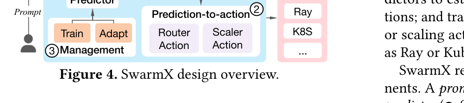
Paper's Figure 4. The system substrate: ① neural predictor consumes the prompt; ② prediction-to-action turns the predicted distribution into a router or scaler action; ③ management trains/adapts predictors; ④ the agent framework binds to existing systems (Ray, K8s). This is the load-bearing overview — every later mechanism is one of these four boxes.



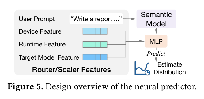
Paper's Figure 5. The core architectural trick: the user prompt goes through a semantic model (isomorphic small variant of the target) to produce semantic features, which the MLP fuses with device/runtime/target-model features to estimate a distribution. Decoupling lets the expensive semantic part be initialized from a pretrained checkpoint while the cheap MLP is the only thing retrained online.



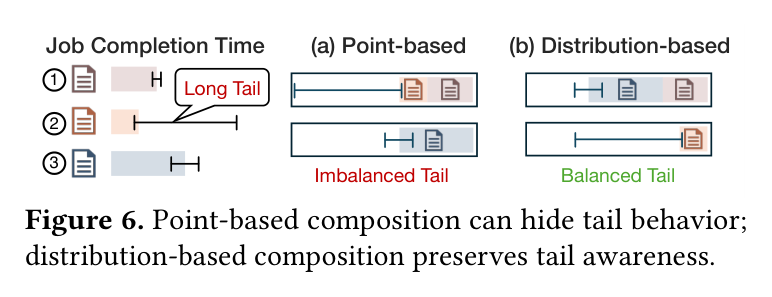
Paper's Figure 6. Reader should notice: point-based composition (a) hides an imbalanced tail and yields a long job-completion tail; distribution-based composition (b) balances the tail. This figure is the visual justification for keeping predictions distributional — the mechanism formalized in §3.2 of the paper and in Algorithm 1 below.

flowchart LR P[Prompt r] --> SM[Semantic model
isomorphic small variant] SM --> SF[Semantic features] DF[Device τ] --> MLP RF[Runtime σ] --> MLP TM[Target-model feat] --> MLP SF --> MLP[MLP] MLP --> D[Quantile distribution D_g] D --> COMP["Q[g] ⊕ D_g"] COMP --> C["C_tail(Q) → cost dist c_g"] C --> S[Sample subset & argmin] S --> ACT["Dispatch/Deploy/Drain"]

The end-to-end data path from prompt to bounded action, added to make the composition-then-sample control flow explicit (the raster figures show pieces but not the full pipeline).

4. 作者证明 #

This is an empirical systems paper: it carries 无形式化作者证明 — 仅实证 (no convergence theorem, variance bound, or optimality proof). What would have been desirable is a bound relating quantile-sketch resolution + composition error to tail-latency regret; the paper instead relies on microbenchmark isolation. However, two learning objectives are formalized and deserve a notation table + physical reading, plus the six minimum checks below.

Notation table #

Symbol	Meaning
$p, m, y$	prompt, target model, observed response property (e.g. output-token length)
$\hat{y}_{p,m}$	semantic model's prediction of that property
$\rho(\cdot,\cdot)$	swappable per-sample loss (MSE / MAE / Huber / pinball)
$x$	feature vector: semantic + target-model + device + runtime
$t$	observed inference time
$\hat q_{\tau_k}(x)$	predicted $\tau_k$-quantile of latency
$\rho_\tau(u)=\max(\tau u,(\tau-1)u)$	pinball (quantile) loss
$w_k>0,\ \sum_k w_k=1$	per-quantile weights
$\oplus$	quantile-grid composition of distributions
$C_{\text{tail}}$	tail-cost evaluator over the full queue state

Loss decomposition — physical meaning #

Semantic-model loss (Eq 1): trains the small isomorphic model to predict a prompt-level property of the target model's response (not the response itself), with a swappable head so the same design serves point or quantile targets.

$$\mathcal{L}_{\text{sem}} = \frac{1}{|\mathcal{D}_{\text{sem}}|} \sum_{(p,m,y)\in\mathcal{D}_{\text{sem}}} \rho\!\left(\hat{y}_{p,m},\, y\right)$$

Router-MLP weighted pinball loss (Eq 2): the MLP directly regresses $K$ quantiles of the inference-time distribution, each weighted, so the output is a full distribution rather than a mean — the enabling condition for tail-aware routing.

$$\mathcal{L}_{\text{router}} = \frac{1}{|\mathcal{D}_{\text{router}}|} \sum_{(x,t)\in\mathcal{D}_{\text{router}}} \sum_{k=1}^{K} w_k\, \rho_{\tau_k}\!\left(t - \hat{q}_{\tau_k}(x)\right)$$

The scaler MLP reuses the identical weighted-pinball form, applied across downstream call-count distributions for all target models — one loss form, two scheduling roles.

Six minimum checks #

1. Units — $t$ in seconds; pinball loss inherits latency units; $\rho_{\tau_k}(t-\hat q)$ is a latency, averaged to a scalar. Consistent.
2. Limiting case — if all $w_k$ mass sits on $\tau=0.5$, Eq 2 reduces to mean-absolute (median) regression, i.e. the point-estimate baseline it is meant to beat. Correctly nests the degenerate case.
3. Monotonicity — pinball loss $\rho_\tau$ penalizes under-prediction ($u>0$) with slope $\tau$ and over-prediction with slope $1-\tau$; higher $\tau$ (tail) penalizes under-estimation more, pushing $\hat q$ upward for tail quantiles. Matches "tail-aware" intent.
4. Quantile monotonicity risk — Eq 2 trains quantiles independently; nothing in the loss forbids crossing ($\hat q_{0.9}<\hat q_{0.5}$). The paper does not prove non-crossing; a practical gap (see §7 关键实现细节).
5. Normalization — $\sum_k w_k=1$ makes $\mathcal{L}_{\text{router}}$ a convex combination of per-quantile losses, so scale is comparable across configs with different $K$. Consistent.
6. Composition sanity — $\oplus$ on quantile grids preserves distribution shape (unlike summing means); composing only the affected entry (Algorithm 1 line 4) then scoring the whole state (line 5) is dimensionally a distribution→distribution→scalar-cost pipeline. Coherent.

Adaptation "proof sketch" (Algorithm 2) #

Per (prompt-class, device) group, accumulate tail pinball error $e=\rho_\alpha(\ell - Q_\alpha(D_p))$ in a sliding window; when the window mean exceeds threshold $\theta$, asynchronously retrain that group's MLP and reset the window. The implicit guarantee is a bounded-lag detector: drift is caught within one window fill, and because only the MLP (not the semantic model) retrains, recovery is cheap — validated empirically at 100 s in §5 (Fig 16).

5. 实验与数据 #



Paper's Figure 8. Router isolated with fixed replica counts. Notice SwarmX is lowest on both, and the striking anomaly: Murakkab, a learned baseline, loses to plain Ray on Text-to-Video because its point-estimate model cannot represent the multi-modal diffusion-iteration latency. The gain is larger on Deep Research (semantic-dependent think/summary latency), confirming the design rationale that wider per-request spread → bigger distribution-aware win.



Paper's Figure 9. Scaler isolated with round-robin routing vs static provisioning. The ~50% Deep Research gain (vs 7.8–13.7% on T2V) tracks structure dynamics: Deep Research varies in both fan-out degree and call depth, so a fixed allocation is frequently misaligned and proactive demand forecasting pays off most.



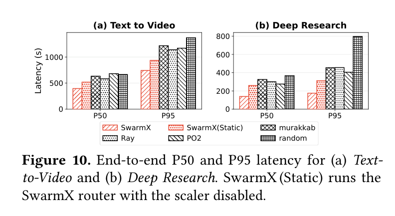
Paper's Figure 10. The load-bearing end-to-end result. The gap between SwarmX and SwarmX (Static) (router only, scaler disabled) isolates the scaler's marginal effect (−20.7% T2V, −43.8% Deep Research P95), demonstrating the router and scaler correct different latency sources and neither alone matches the full system.



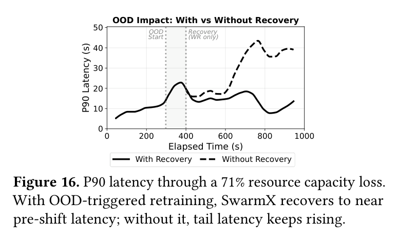
Paper's Figure 16. Robustness evidence. Without adaptation the stale predictor misroutes and P90 climbs past 40 s; with OOD-triggered MLP retraining SwarmX detects the shift and holds P90 below 20 s, with detection+retraining completing within 100 s — the empirical stand-in for the missing formal convergence guarantee.

Overhead (Table 2) — the cheapness that lets prediction sit on the online path:

	Wan2.1-T2V-1.3B	Qwen3-8B
Served-model latency	17–137 s	0.7–100+ s
Prediction time	<1 ms	30 ms (CPU), ~4 ms (GPU)
Memory	261 KB (66K params)	~100 MB (35M params)

Prediction is 3–4 orders of magnitude cheaper than the served model, so it can be colocated with execution without becoming the bottleneck.

Semantic-model sizing (Fig 14 / §5.5): sweeping parameter-reduced isomorphic Qwen3 variants, output-length prediction error drops sharply then saturates; the 35M model sits at the knee (error 27.89), so SwarmX picks the smallest variant past the knee — the accuracy–overhead search made concrete.

Dataset / workloads (Table 1): seven services in three difficulty tiers — structured pipelines (Deep Research on 20k DR-Bench samples; Text-to-Video on 2k OpenVid-1M), open-ended agentic (OpenClaw on MCP-Atlas; Coding Agent on a SWE-bench-Pro trace), and production (Video OCR, Video Transcode, Entity Semantic Analysis) with ~11M real serving records. Training records log prompt context, target-model info, device/runtime features, prediction, scheduling decision, and observed outcome; optimizer is AdamW to convergence.

Where it ties, not wins: on single-model Coding Agent P95, SwarmX only "maintains similar performance" — its workload distribution is more homogeneous, so distribution-awareness has less tail to exploit. Honest negative signal consistent with the design thesis.

6. 论证链 #

#	Step	Support (paper-internal)
1	Prompt semantics drive both inference time and call structure, with heavy-tailed/multi-modal distributions.	Figs 2–3: 194/886/1569 tokens; $S_1/S_2/S_3$ call structures; cross-model, cross-workload spread.
2	Point-estimate schedulers (Ray heuristics, Murakkab averages, PSC/Cilantro regressors) cannot represent that spread, so tail decisions are poor.	§2.3 argument + Fig 8: Murakkab loses to Ray on T2V.
3	A small isomorphic variant of the target predicts prompt-level response properties cheaply; a tiny MLP fuses device/runtime features to output a quantile distribution.	§3.1 + Fig 5; Eqs 1–2; Fig 14 sizing (35M at knee).
4	Keeping predictions distributional and composing with $\oplus$, then scoring the whole state with $C_{\text{tail}}$ and sampling, protects the tail better than composing point estimates.	Fig 6; Algorithm 1; §5.2 wider-spread→bigger-gain trend.
5	Router (request-time) and scaler (structure-aware provisioning) correct different latency sources and are complementary.	Fig 10 SwarmX-vs-SwarmX(Static) gap.
6	An OOD sliding-window monitor retraining only the MLP keeps accuracy under drift at low cost.	Algorithm 2; Fig 16 (71% loss → 100 s recovery).
7	Gains hold at production scale and even on non-AI CPU services with input-dependent latency.	§5.4: 2× throughput, P99 −44–52%, Video OCR/Transcode.

7. 实现 cross-reference #

[实现未公开] at the time of the L1 — the paper states SwarmX is "soon-to-be open-sourced" (§8) but no repository/file:line is disclosed. The following are the reproducibility anchors and easy-to-miss tricks.

核心技术壁垒 (dedicated paragraph): the enabling insight is architectural isomorphism, not merely "use a small LM". SwarmX instantiates parameter-reduced variants that preserve the Qwen3 architectural shape (fewer layers / narrower layers) and initialize from a pretrained checkpoint, then replace the final layer with an output-length / structure head. This is why a 35M model can proxy an 8B target's response properties: it shares the inductive biases of the family it predicts. Reproducing SwarmX without this — e.g. training a generic small LM from scratch — would forfeit both the accuracy and the near-zero training cost, and the sizing sweep (Fig 14) would land at a much larger, slower predictor. The second pillar is that predictions are never collapsed to a mean before the final decision: quantile sketches + $\oplus$ composition + tail-cost sampling is the machinery that turns "we know the distribution" into "we route/scale for the tail".

关键实现细节 (easy-to-miss tricks):

1. Scaler load offload — one scaler may cover many services, so SwarmX delegates heavy prompt parsing to upstream routers and feeds the scaler only the resulting prompt-aware representation + a lightweight MLP; this preserves prompt awareness while keeping scaler-side prediction cheap (§4). Miss this and the scaler becomes a prediction hotspot.
2. Deployment-change threshold — the scaler applies a hysteresis threshold before committing deploy/drain so it does not thrash on small demand fluctuations (§3.2). Also note quantiles are trained independently (Eq 2), so an implementation must guard against quantile crossing — the paper does not enforce non-crossing.
3. Predictor colocation + fallback — predictors are colocated with worker servers (not control servers) under eventual-consistency weight distribution; on predictor failure SwarmX falls back to the underlying scheduler policy so prediction is never on the critical availability path (§4).

Reproducibility / ecosystem: no open training code released yet; closest open references for the RL-free supervised quantile-regression recipe are standard PyTorch + AdamW pipelines (the pinball loss is off-the-shelf). Serving stack is public: vLLM 0.16.0 / SGLang workers under Ray, so the host infrastructure is reproducible even though the predictor training corpus (~11M production records) is not. Pythia (arXiv:2604.25899) is the acknowledged parallel effort predicting workflow structure — but without prompt-semantic modeling, making it the nearest community reimplementation target for the structure half of the problem.