Knowing When to Ask for Help: Bayesian Self-Escalation in Hierarchical LLM Agents
Knowing When to Ask for Help: Bayesian Self-Escalation in Hierarchical LLM Agents — L2 #
1. TL;DR #
A junior LLM keeps an online Bayesian posterior $B_t$ over whether its own final answer will be correct, updated $O(1)$ per token from uncertainty signals, and escalates to a senior model the moment $B_t$ drops below a cost-derived threshold. Core theorem: escalation quality is bound by posterior calibration, not decision-rule cleverness.
2. Q1 / Q2 / Q3 #
Q1 — 痛点 (what problem) #
LLM hierarchies route at the wrong time. *Routing before generation throws away the information that accrues while the junior model reasons; routing after full generation wastes compute on a response that gets discarded anyway. Neither exploits the fact that, token by token, a junior model emits a stream of uncertainty evidence that progressively reveals whether it is on track. The question "should I hand this off, and when?" is a sequential decision, but prior cascades (FrugalGPT, RouteLLM) and agreement-based methods answer it only at response granularity* and often need multiple full samples.
A second, subtler pain point: raw uncertainty is not a decision signal. High token entropy does not mean the answer is wrong, and low entropy does not mean it is right — a model can be confidently wrong. So thresholding raw entropy mid-stream is unprincipled.
Q2 — 方法 (the method) #
Frame mid-generation handoff as an optimal-stopping problem over a learned competence posterior. Define $B_t = \mathbb{P}(Y=1 \mid \mathcal{F}_t)$, the probability the junior's eventual answer is correct given signal history $\mathcal{F}_t$. Under a conditional-i.i.d. signal model (Assumption 1), the belief update collapses to a running log-odds sum $\ell_t = \ell_0 + \sum_s \lambda(e_s)$ (Lemma 1) — a one-line sequential Bayes filter. Compare the forward cost of escalating now vs. finishing locally and you get a closed-form myopic threshold (Proposition 1) and a dynamic-program optimal policy (Theorem 2) that provably has threshold structure.
核心技术壁垒 (the single hardest-to-replicate insight): the paper proves — via Proposition 3 and Corollary 1 — that regret over the oracle is bounded by $L \cdot \mathbb{E}|B_t - \hat B_t|$, i.e. by the calibration error of the posterior, independent of how clever the decision rule is. This reframes the entire engineering problem: do not tune the router, calibrate the belief (Brier score, not ECE, is the right target). Replicating the mechanism is easy; internalising and correctly exploiting this reduction — including that Brier (not ECE) is the correct optimisation objective and that direct end-to-end policy learning destroys the guarantee — is the defensible contribution.
Q3 — 结果 (what was shown) #
- Simulation (40k queries, known ground truth): Bayesian optimal-stopping hits 96.0% accuracy escalating only 40% of queries, vs. 91.0% for a tuned fixed-rule and 90.1% for always-escalate, at lower cost (Table 1).
- Real models (Qwen2.5-Coder 1.5B→7B on MBPP, 257 tasks): cumulative-belief AUROC rises 0.51 → 0.76 over generation; streaming escalation reaches 74.7% accuracy at 0.98× junior-only compute, dominating post-hoc routing (which needs 1.41×).
- 2 of 3 pre-registered predictions confirmed (the calibration-regret prediction (c) was left for the controlled simulation, not the real-model run).
3. 架构 / 方法图 — the agent loop #
The "agent" here is a single junior that runs a tight observe → update-belief → decide loop per token, with a one-way escalation transition to the senior. The method decomposes into an online path (cheap, per-token) and an offline path (expensive, done once).
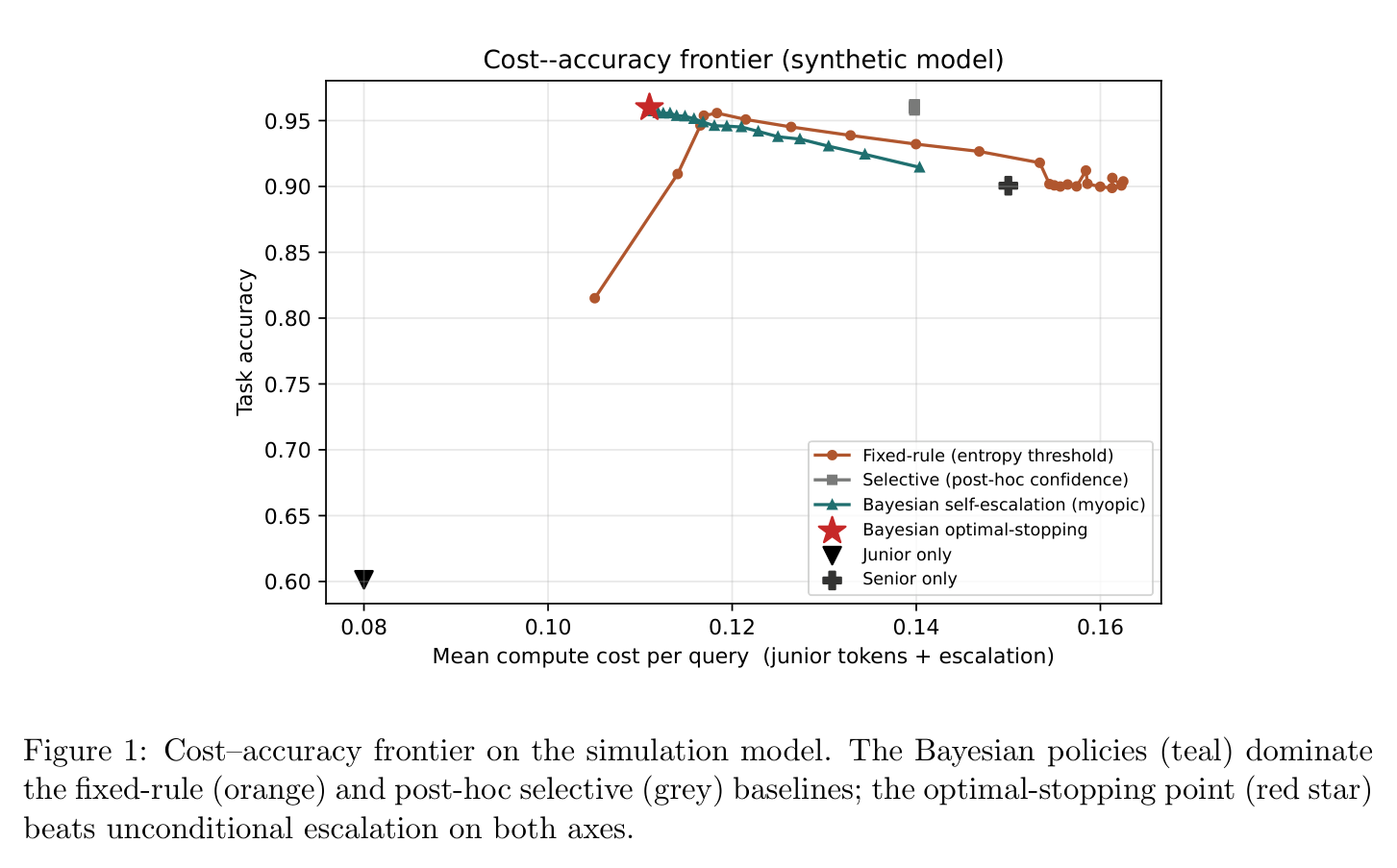
Figure 1 — the cost–accuracy frontier from the 40k-query simulation. Bayesian policies (myopic, constant, optimal-stopping) form the upper-left envelope, dominating the fixed-rule and post-hoc selective baselines across the whole frontier; the optimal-stopping operating point beats unconditional escalation at strictly lower cost. This is the headline "the belief-driven policy Pareto-dominates" claim in one picture.
The per-turn agent loop and the memory/escalation transition:
- Memory model: short-term = the running log-odds scalar $\ell$ (the entire belief state is one number); the junior's generation trace, tool-call history and retrieved evidence are the long-term artifacts handed off on escalation. There is no vector DB — the belief is a sufficient statistic of the signal history.
- Tool/handoff invocation:
DistillContextproduces text-level artifacts (partial reasoning, scratchpad, tool-call log, retrieved evidence), not hidden activations. This is deliberate: junior and senior may differ in architecture, tokenizer and KV-cache layout, so the senior cannot ingest hidden states. The re-reading cost is folded into the escalation charge $\gamma$. - Error / fallback: escalation is the fallback. It is a one-way, terminal transition — once the agent escalates it never returns to the junior. If the belief never crosses the threshold, the agent falls through to
J.finalize()at horizon $T$. - Planning style: not ReAct or tree search — a predetermined optimal-stopping schedule $\{\tau_t\}$ computed offline by backward induction. There is no backtracking; the only decision each step is the binary continue/escalate.
4. 作者证明 #
This is a theory paper with a full formal development (not 仅实证). Notation table and the load-bearing equations, then the minimum checks.
Notation table #
| Symbol | Meaning |
|---|---|
| $Y \in \{0,1\}$ | latent event: junior's completed answer is correct |
| $\pi = \mathbb{P}(Y=1)$ | base competence prior |
| $e_t$ | per-step raw signal (token entropy, next-token margin, probe) |
| $\mathcal{F}_t = \sigma(e_1,\dots,e_t)$ | filtration (signal history) |
| $B_t = \mathbb{P}(Y=1\mid\mathcal{F}_t)$ | competence posterior (the belief) |
| $\lambda(e) = \log[f_1(e)/f_0(e)]$ | per-step log-likelihood ratio |
| $\ell_t = \log[B_t/(1-B_t)]$ | belief in log-odds |
| $\kappa,\ \gamma,\ L,\ q$ | junior per-step cost, escalation cost, wrong-answer cost, senior success prob |
| $\tau_t^{\mathrm{myo}},\ \tau_t^\star$ | myopic / optimal threshold at step $t$ |
| $C$ | Chernoff information between $f_0,f_1$ |
Load-bearing equations & physical meaning #
Belief filter (Lemma 1): $\ell_t = \ell_0 + \sum_{s=1}^{t} \lambda(e_s)$, with $B_t = \sigma(\ell_t)$. Physical meaning: the belief is a sequential Bayesian filter; each token increments the log-odds by its evidence $\lambda(e_s)$, so the per-token update is $O(1)$ — a table lookup plus an add. This is what makes the method cheap enough to run inside the generation loop.
Myopic threshold (Proposition 1): escalate iff $B_t < \tau_t^{\mathrm{myo}}$ where
$$\tau_t^{\mathrm{myo}} = q - \frac{\gamma}{L} + \frac{(T-t)\kappa}{L}$$
Physical meaning: escalate readily when the senior is reliable (large $q$), errors are costly (large $L$), and escalation is cheap (small $\gamma$). The term $(T-t)\kappa/L$ makes early tokens (many steps remaining) more eager to escalate because finishing locally is still expensive.
Optimal DP (Theorem 2 / §4.2): $V_t(b) = \min\{\gamma+(1-q)L,\ \kappa + \mathbb{E}[V_{t+1}(B_{t+1})\mid B_t=b]\}$. Physical meaning: the second branch captures the option value of waiting — even though the belief is a martingale, the nonlinearity of $V$ means a later token can lower expected future cost.
Calibration-regret bound (Proposition 3, at $\tau_t^{\mathrm{myo}}$): $\mathrm{Regret}_t \le L\cdot\mathbb{E}[|B_t - \hat B_t|]$, tightened by Corollary 1 to $\mathrm{Regret}_t \le L\sqrt{\mathrm{BS}(\hat B_t)-\mathrm{BS}(B_t)}$. Physical meaning: the whole gap to the oracle is the posterior's excess Brier score — the binding constraint is calibration, not the decision rule.
6 minimum checks #
- Dimensional/units check — $\tau_t^{\mathrm{myo}}$ is a probability (dimensionless): $q$ is a probability, $\gamma/L$ and $(T-t)\kappa/L$ are cost-over-cost ratios → all dimensionless. ✓ Consistent.
- Boundary/terminal check — at $t=T$, $(T-t)\kappa/L \to 0$ so $\tau_T^{\mathrm{myo}} = q - \gamma/L$, matching both the DP terminal value $V_T$ and the optimal $\tau_T^\star = q-\gamma/L$. ✓ The three derivations agree at the horizon.
- Monotonicity check — Theorem 2's proof needs each $V_t$ non-increasing in $b$. Escalate branch is constant in $b$; continue branch is non-increasing by Lemma 2 (FOSD-monotone transition); min of two non-increasing functions is non-increasing → escalate set is a lower interval $[0,\tau_t^\star]$. ✓ Internally closed.
- Martingale consistency (Theorem 1) — $\mathbb{E}[B_{t+1}\mid\mathcal{F}_t]=B_t$ follows from the tower property on $B_t=\mathbb{E}[\mathbf 1\{Y=1\}\mid\mathcal{F}_t]$. ✓ And it does not contradict waiting having value (Remark 2, option-pricing analogy) — value comes from nonlinearity of $V$, not drift.
- Asymptotic/rate check — Proposition 2 gives exponential belief separation $e^{-tC}$, and Theorem 3 gives plug-in regret $O(1/\sqrt{m})$; the simulation measures a log-log slope of $-0.53$ vs. the predicted $-0.5$. ✓ Rate matches to within sampling noise.
- Self-consistency / retraction audit — the authors themselves flag that (a) thresholds are not monotone in $t$ (Remark 4 retracts $\tau_1^\star\le\dots\le\tau_T^\star$ with a counterexample) and (b) the calibration bound only holds at $\tau_t^{\mathrm{myo}}$ (Remark 5 retracts the all-$\tau$ version, counterexample $\tau{=}0.5, B_t{=}0.49, \hat B_t{=}0.51$ gives regret 0.26 ≫ 0.02). ✓ The published proofs survive these corrections; the extra $|g_t(\tau)|\mathbb{P}(D)$ term is retained away from the myopic point.
- Online inference loop — Algorithm 1 (§6): per token,
ℓ ← ℓ + λ̂(e_t); B ← σ(ℓ); escalate whenB < τ_t, callingDistillContext(trace_{1:t}, tool_state, evidence)thenS.solve(x, c). The signale_tis token entropy / next-token margin / probe output. - Offline schedule — Algorithm 2 (§6): backward induction from the DP terminal value
V(b_j) = min{γ+(1-q)L, (1-b_j)L}, propagating beliefs under both class-conditionals to getτ_t^★ = max{b_j : γ+(1-q)L ≤ C(b_j)}. - Real-model harness (§8, §11 Reproducibility): one harvest script (run junior on MBPP, record
(e_{1:T}, Y)via unit-test execution) + three analysis scripts (separation/frontier, streaming escalation, $B_t$ AUROC). Posterior fit by logistic regression on running means of three signals with 5-fold CV (all beliefs out-of-fold). - Per-step isotonic recalibration beats the plug-in filter in deployment (§5.5 Remark): recalibrating $\hat B_t$ directly each step targets $\mathbb{E}|\hat B_t-B_t|$ without the linear-in-$t$ error compounding that the plug-in LLR estimator suffers; the $1/\varepsilon$ term in Theorem 3 is pessimistic because it charges for low-mass bins the belief rarely visits.
- One $\hat\lambda$, many schedules (§6 task adaptivity): per-domain priors $\pi_d$ and cost tuples yield per-domain thresholds from the same fitted signal model via a cheap re-run of Algorithm 2 — no refitting. When senior price, latency, or reliability $q$ changes, you rerun backward induction only, never retrain the posterior.
Weakest link: Assumption 1 (signals conditional-i.i.d.) is acknowledged false for real token streams (§10). Lemma 1's exact filter degrades to an approximation; the threshold structure (Lemma 2) survives for any density pair, but the belief values require a sequence model of the signal to stay calibrated.
5. 实验与数据 #
Simulation — matched-compute slice #
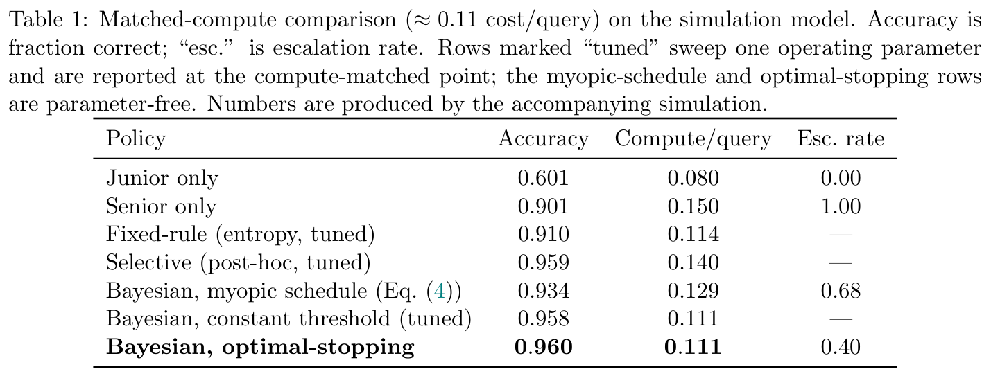
Table 1 — all policies sliced at ≈0.11 cost/query. Bayesian optimal-stopping reaches 96.0% accuracy at a 0.40 escalation rate, beating fixed-rule (91.0%) and matching/beating the tuned post-hoc selective baseline at lower cost. The literal myopic schedule over-escalates (68% rate) because its first-token threshold $\tau_1^{\mathrm{myo}}=0.828$ sits above the prior $\pi=0.60$ — the reader should notice the myopic rule is suboptimal precisely where option value matters most, motivating the full DP.
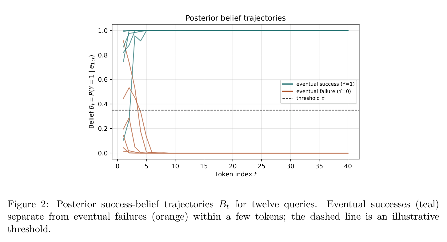
Figure 2 — belief dynamics. Eventual successes (teal) drift up, failures (orange) drift down, visually confirming Proposition 2's exponential separation. The computed threshold schedule hugs low interior values (0.02→0.08) then jumps to $q-\gamma/L=0.75$ exactly at the horizon — a direct picture of Remark 4's non-monotonicity: option value keeps interior escalation conservative, remaining-token cost only bites near the end.
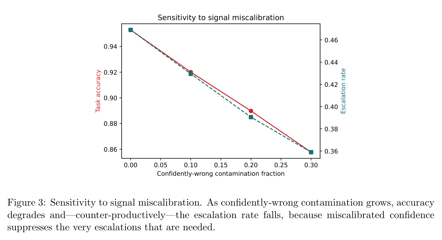
Figure 3 — the calibration-is-binding experiment. As confidently-wrong contamination rises 0% → 30%, accuracy falls 95.2% → 85.7% and the escalation rate drops 0.47 → 0.37. This is the counterintuitive core result: miscalibrated confidence suppresses the escalations most needed, operationalising the $O(L)$ regret event of Proposition 3 (and serving as the controlled analogue of untested prediction (c)).
Robustness across signal models #
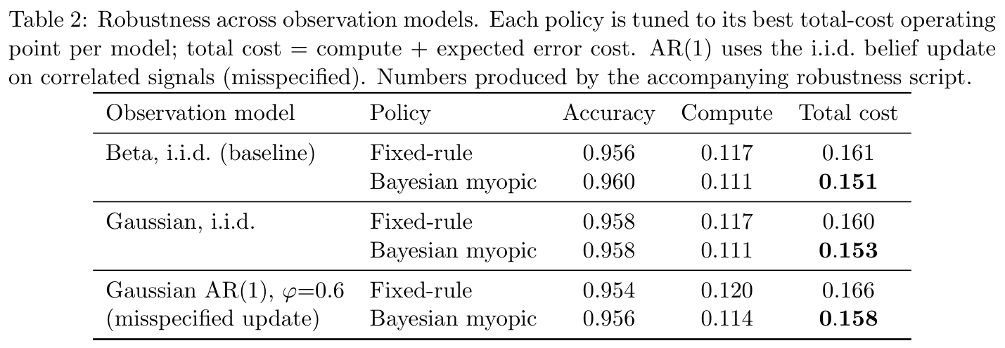
Table 2 — Beta i.i.d., Gaussian i.i.d., and misspecified Gaussian AR(1). The Bayesian policy attains the lowest total cost in all three; under AR(1) (Assumption 1 violated) the edge narrows but does not invert (0.158 vs. 0.166), so the method degrades gracefully rather than breaking when its i.i.d. assumption fails.
Real-model validation (MBPP, Qwen 1.5B→7B) #
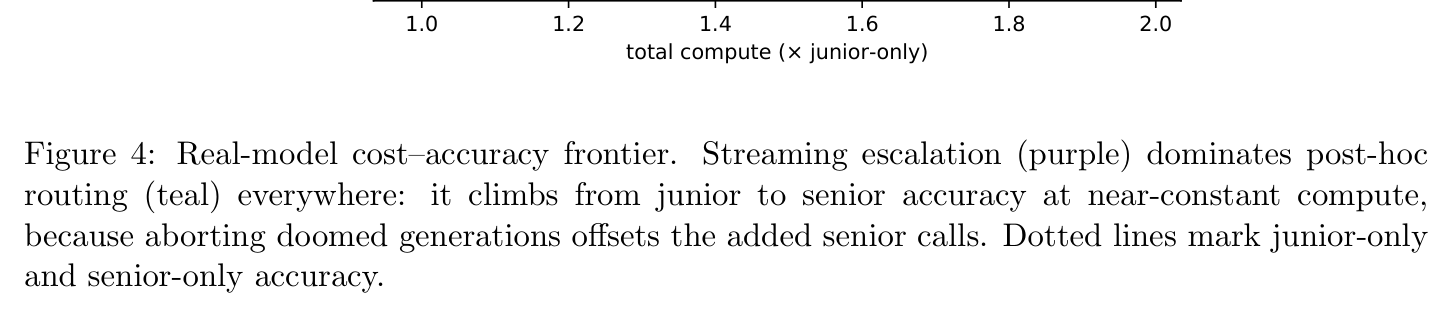
Figure 4 — streaming vs. post-hoc on real models. Streaming escalation dominates post-hoc routing everywhere; to reach 75% accuracy it uses 30.2% less total compute (14,841 vs. 21,273 tokens) and lands at essentially junior-only cost. The advantage is structural: post-hoc pays for full junior generation before routing, streaming stops paying the moment the belief turns against it.
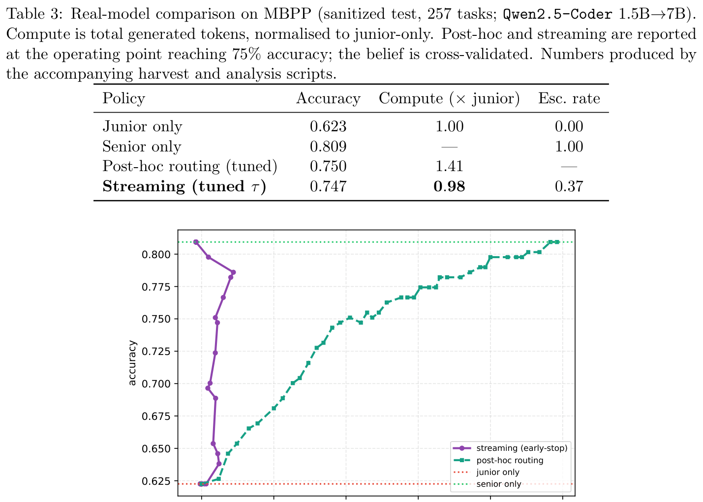
Table 3 — the real-model operating points. Streaming at tuned $\tau$ reaches 74.7% accuracy at 0.98× junior compute / 0.37 escalation rate, versus post-hoc routing's 75.0% at 1.41×. Junior alone is 62.3%, senior alone 80.9%, so streaming captures most of the gap at near-zero extra compute — the tight ≈1.0× cancellation (saved aborted tokens ≈ senior overhead) is the surprising practical headline.
Supporting discrimination curve:
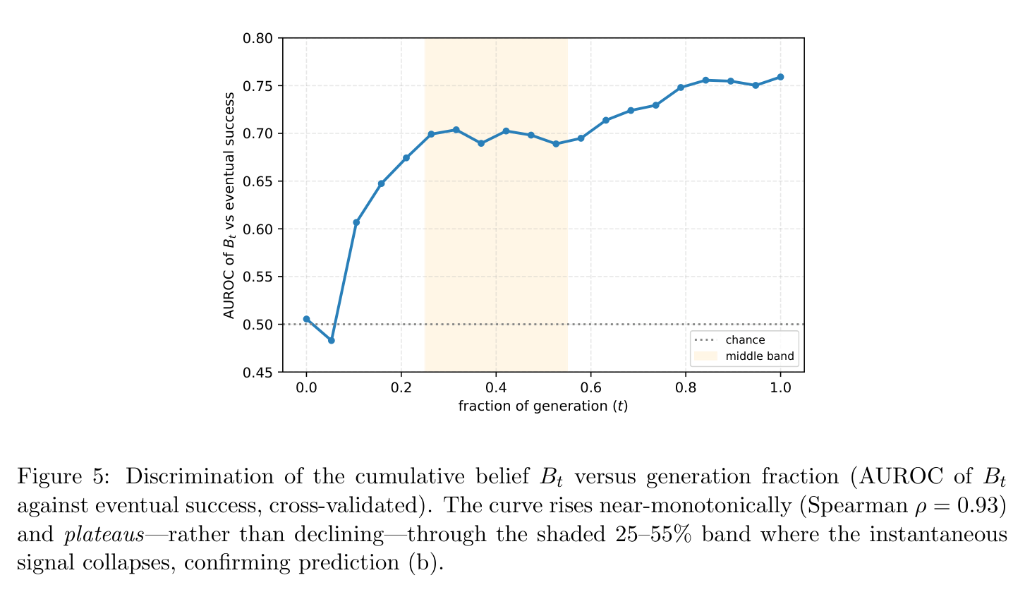
Figure 5 — AUROC of $B_t$ rising 0.51 → 0.76 (Spearman ρ=0.93 with generation fraction). Crucially it plateaus, not declines, through the 25–55% band where the instantaneous entropy signal collapses (confident-wrong failures mix with hard-but-correct successes) — confirming pre-registered prediction (b) and validating the "accumulate calibrated belief rather than react per-step" design.
6. 论证链 (paper-internal) #
| # | Step | Depends on | Conclusion |
|---|---|---|---|
| 1 | Define competence posterior $B_t=\mathbb{P}(Y{=}1\mid\mathcal{F}_t)$ and assume conditional-i.i.d. signals (Assumption 1) | §3 setup | Belief is a well-defined probability object over eventual correctness |
| 2 | Derive belief update as log-odds sum (Lemma 1) | Step 1 | Update is $O(1)$ per token → cheap enough to run inside generation |
| 3 | Write forward-cost comparison (escalate vs. finish) → myopic threshold (Proposition 1) | Steps 1–2, cost model §3.1 | Closed-form, parameter-free escalation rule |
| 4 | Pose the full cost-to-go DP and prove transition is FOSD-monotone (Lemma 2) | Step 2 | Continue-value is non-increasing in belief |
| 5 | Backward induction → optimal policy has threshold structure (Theorem 2), using monotonicity only | Steps 3–4 | Optimal policy = escalate iff $B_t\le\tau_t^\star$; robust (no concavity needed) |
| 6 | Bound regret of a miscalibrated plug-in belief (Proposition 3 → Corollary 1) | Steps 3,5 | $\mathrm{Regret}_t \le L\sqrt{\mathrm{BS}(\hat B_t)-\mathrm{BS}(B_t)}$ — calibration is binding |
| 7 | Finite-sample regret of plug-in LLR (Theorem 3) | Step 6 | Regret decays $O(1/\sqrt{n})$ in calibration trajectories |
| 8 | Instantiate as Algorithms 1 (online) + 2 (offline schedule), validate in simulation (§7) and on MBPP (§8) | Steps 2–7 | 2/3 pre-registered predictions confirmed on real models |
7. 实现 cross-reference #
公开代码: github.com/nadeem-shaikh/llm-self-escalation (full pipeline) and Zenodo DOI 10.5281/zenodo.21330787 (paper + simulation scripts). Line-level citations are not available from the L1, so references below are to the paper's algorithm listings and the released script set.
核心技术壁垒 (dedicated paragraph) #
The replication barrier is not the mechanism — the belief filter is a running sum and the schedule is textbook backward induction. The barrier is the reduction that calibration, measured by Brier score, is the binding constraint (Proposition 3 → Corollary 1). This dictates every non-obvious engineering choice: calibrate the posterior with isotonic regression / temperature scaling targeting Brier (Remark 6 shows small ECE is insufficient — a belief can be calibrated-on-average while ignoring information); keep posterior and thresholds modular rather than learning an escalate/continue policy end-to-end (which would destroy both the $O(1/\sqrt n)$ guarantee and the auditability of $\hat B_t$); and treat the senior handoff as text, not activations, so the method is tokenizer-agnostic. A team that copies Algorithm 1 but trains the router end-to-end on raw entropy will silently forfeit the theorem and hit the confidently-wrong suppression failure of Figure 3.