Latency-Aware Orchestration for Multi-Agent LLM Workflows on Heterogeneous GPUs — L2 #

1. TL;DR #

A prediction-guided runtime turns concurrent multi-agent workflows into a

mutable physical execution graph: it forecasts per-(model,request,device)

cost, fuses same-deployment chains, coalesces model lifecycle actions across

workflows, and jointly schedules placement/order/lifetime under a live

heterogeneous pool — cutting burst makespan by 36.8% and saving up to

24.63 GPU-s/session.

2. Q1 / Q2 / Q3 #

Q1 — 痛点 (problem) #

Concurrent multi-agent workflows run on **small, fixed, heterogeneous GPU

pools** (private/cost-constrained deployment). Prior workflow schedulers act

on individual model calls once ready: they can reorder priority but cannot

(a) manage when a downstream model becomes available and (b) preserve

physical continuity across logical node boundaries. Two measured

consequences dominate:

• Model-availability delay accounts for 77.3–85.5% of request waiting

under Parrot and Kairos; **model loading consumes more GPU time than token

generation**, and idle residency adds another 28.1–33.0% of GPU time.

• Repeated physical admission at same-model node boundaries produces a

large tail: 39–42% of the p95 session (97.1–155.1 s) is spent

re-releasing/re-acquiring the backend at boundaries where the successor

needs the same deployment.

Q2 — 方法 (method) #

Separate logical semantics (what must happen, which results are visible)

from state-dependent physical execution (scheduling unit, model-lifecycle

action, resource order, placement). Three stages operate on a bounded

planning window $\mathcal{W}_t$ of ready + immediate near-ready units:

1. Predictor — maps (model op-graph, request config, device attrs) →

$(\widehat{T}^{\text{run}}, \widehat{M}^{\text{peak}}, \widehat{T}^{\text{load}})$ via a graph encoder + 3 target heads, cached into buckets and propagated through dependencies to forecast release times.

2. Constructor — workflow-local fusion of strictly-linear

same-deployment chains, then cross-workflow coalescing of compatible

lifecycle actions (one load/prefetch serves multiple isolated workflows),

inducing an implicit candidate space $\mathcal{G}_t$.

3. Scheduler — event-driven heuristic that jointly picks

lifecycle/replica/device bindings and resource order on one predicted

timeline, ranks plans by a lexicographic key $\Phi_t$, commits only the

next executable prefix, and replans the uncommitted suffix from feedback.

核心技术壁垒: the joint, cumulative-memory-feasible online construction

of the graph and its schedule together — evaluating each transformation's

cumulative effect on ready work, scarce devices, transient memory, and

resident state at every predicted transition boundary (Eq 11), rather than

scoring transformations in isolation. This is what no prior planner does.

Q3 — 结果 (results) #

• Burst: makespan 634.2 s (−35.8%/−36.8% vs Parrot/Kairos), overall p95

587.0 s (−25.4–25.9%).

• Lowest makespan at both Poisson rates (−12.4–13.1% and −1.6–6.6%), but

honestly loses some Poisson p95/model-scoped tails (global objective

trades a local tail for earlier drain).

• Up to 24.63 GPU-s/session saved, driven mostly by cut idle residency.
• Predictor: 8.05% loading WAPE, 7.25% runtime WAPE, 97.94% ordering / 97.82%

window-fit decision accuracy.

3. 架构 / 方法图 #



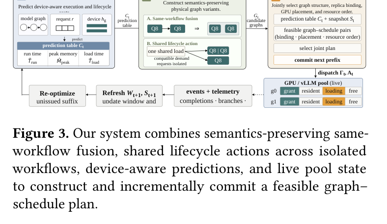
*Paper's Figure 3 (caption: "Our system combines semantics-preserving

same-workflow fusion, shared lifecycle actions across isolated workflows,

device-aware predictions, and live pool state to construct and incrementally

commit a feasible graph–schedule plan.").* This is the load-bearing

architecture figure: it shows the Predictor→Constructor→Scheduler pipeline

feeding on live pool snapshot $S_t$ and committing only a prefix, so the

reader should notice the incremental commit + replan loop rather than a

one-shot planner.



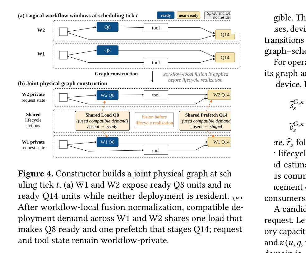
*Paper's Figure 4 (caption: "Constructor builds a joint physical graph at

scheduling tick $t$. (a) W1 and W2 expose ready Q8 units and near-ready Q14

units while neither deployment is resident. (b) After workflow-local fusion

normalization, compatible deployment demand across W1 and W2 shares one load

that makes Q8 ready and one prefetch that stages Q14; request and tool state

remain workflow-private.").* This figure is the clearest illustration of the

central mechanism: fusion happens before lifecycle realization, and a

single load/prefetch is shared across two isolated workflows while each

workflow's request/tool state stays private — the source of the dominant

makespan benefit measured later.

The construction/commit loop can also be read as a sequence per scheduling

tick:

flowchart LR W["Planning window W_t
ready F_t + near-ready N_t"] --> P[Predictor: release + device costs] P --> C["Constructor: fuse chains
coalesce lifecycle actions"] C --> S["Scheduler: rank plans by Phi_t
check Eqs 9-11"] S --> X[Commit next prefix] X -->|"arrival / completion / telemetry"| W

4. 作者证明 #

This is a systems paper: 无形式化作者证明 — 仅实证. There is no

convergence theorem, regret bound, or optimality proof. What exists instead

is a feasibility construction — a set of invariants and constraints that

any accepted plan must satisfy — plus a lexicographic ranking objective. A

desirable-but-absent guarantee would be a competitive-ratio bound of the

online heuristic against the trace-conditioned Oracle it compares to.

Notation table (load-bearing symbols) #

Symbol	Meaning
$L_t = \bigcup_{w} L^w_t$	union of resolved workflow portions at time $t$
$G^0_t = \text{Fuse}(L_t)$	fusion-normalized graph
$F_t,\ N_t$	ready / near-ready unit sets
$\mathcal{W}_t = G^0_t[F_t \cup N_t]$	planning window
$G^p_t = \langle U^0_t \cup H^p_t, E^{L,p}_t\rangle$	a physical realization
$H^p_t$	device-symbolic load / prefetch / reclaim actions
$d(u),\ m(u)$	deployment identity / model of unit $u$
$\mathcal{G}_t$	admissible physical-realization candidate space
$\widehat{r}_u,\ \widehat{c}_v$	predicted release / completion
$\Phi_t(G,\pi)$	lexicographic ranking key

方程物理意义 + 6 minimum checks #

1. Eq 1 $\left(\widehat{T}^{\text{run}}_{m,r,g}, \widehat{M}^{\text{peak}}_{m,r,g}, \widehat{T}^{\text{load}}_{d,g}\right) = \text{Predict}(\mathcal{G}_m, r, h_g)$ — three separate heads; loading depends on deployment+device only, run/peak on request too. Check: dimensionality is per-(model,request,device), not workflow-level — this is what makes cross-device ranking possible.
2. Eq 2 release $\widehat{r}_u = t$ if $u\in F_t$, else $\max_{v\in\text{pred}}\widehat{c}_v$. Check: near-ready units release when the slowest predecessor finishes (max, not min) — correct lower bound on start.
3. Eq 3 fusible-chain condition (one-to-one adjacency, same $d$, config-compatible). Check: the one-to-one succ/pred constraint forbids fusing across a branch/join, so contraction cannot violate a dependency.
4. Eq 4 $I^{\text{adm}}_c = \max_i I_i$, $O^{\text{adm}}_c = \max_i O_i$, $\widehat{T}^{\text{run}}_{c,g} = \sum_i \widehat{T}^{\text{run}}_{m(c),r_i,g}$. Check: admission reserves the max context (pessimistic, safe) but predicts release as the sum of runtimes (sequential under one lease) — the asymmetry is deliberate and consistent.
5. Eq 5 $H^X_t(u) = \{\langle\alpha_X(d(u))\rangle, \langle\text{Reclaim}, \alpha_X(d(u))\rangle\}$ with $\alpha_F=\text{Load}$, $\alpha_N=\text{Prefetch}$. Check: exactly two lifecycle shapes per class (direct vs reclaim-then-load); ready→Load, near-ready→Prefetch is the correct eager/lazy split.
6. Eq 11 cumulative memory: $R^{G,\pi}_{a,t}(\tau) + \sum_s x_{s,a} M^{\text{inc}}_{s,a}\mathbb{1}[\widehat{s}_s \le \tau < \widehat{c}_s] \le C^M_a,\ \forall a,\tau$. Check: the indicator sums only concurrently-active requests at each transition instant $\tau$, so it catches transient overload during a load/reclaim even when the steady-state resident set fits — the crux of feasibility.

Additional constraints tying selection to placement (Eq 9), resource-order

orientation (Eq 10), and feasible device domain (Eq 8) complete the

admissible-domain definition; the objective is Eq 12:

$$\Phi_t(G, \pi) = \left(-A_1, \dots, -A_K,\ \widehat{C}_F,\ -P_N,\ H^{\text{life}}\right)$$

Physical meaning: lexicographic — first maximize admitted ready work per

priority class ($-A_k$), then minimize latest ready completion $\widehat{C}_F$,

then maximize timely prefetches $-P_N$, then minimize lifecycle overhead

$H^{\text{life}}$. Ready work is never sacrificed for prefetch.

5. 实验与数据 #



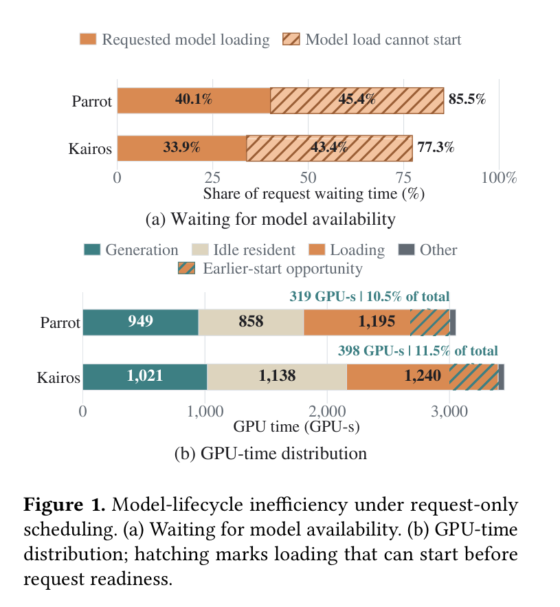
*Paper's Figure 1 (caption: "Model-lifecycle inefficiency under request-only

scheduling. (a) Waiting for model availability. (b) GPU-time distribution;

hatching marks loading that can start before request readiness.").* This

motivation figure is load-bearing: (a) shows model-availability delay is

77.3–85.5% of waiting, and (b) shows loading > generation GPU time with

28.1–33.0% idle residency — establishing that priority reordering alone

cannot help, since the bottleneck is lifecycle, not ordering.



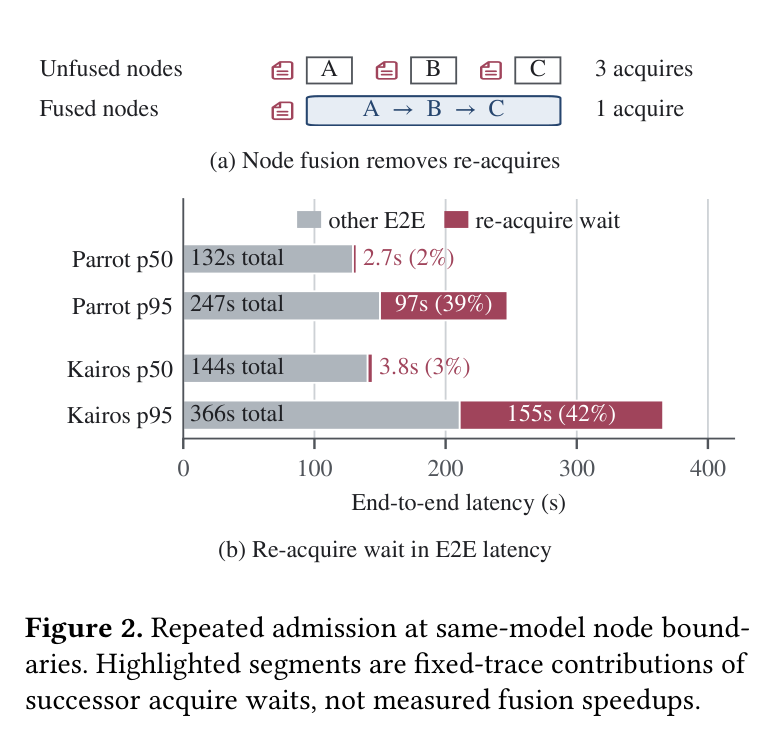
*Paper's Figure 2 (caption: "Repeated admission at same-model node

boundaries. Highlighted segments are fixed-trace contributions of successor

acquire waits, not measured fusion speedups.").* Notice the tiny median

(2.7–3.8 s, 2–3%) versus a huge tail (97.1–155.1 s, 39–42% of the p95

session) — this asymmetry is precisely what fusion targets by keeping a

same-deployment chain under one backend admission.



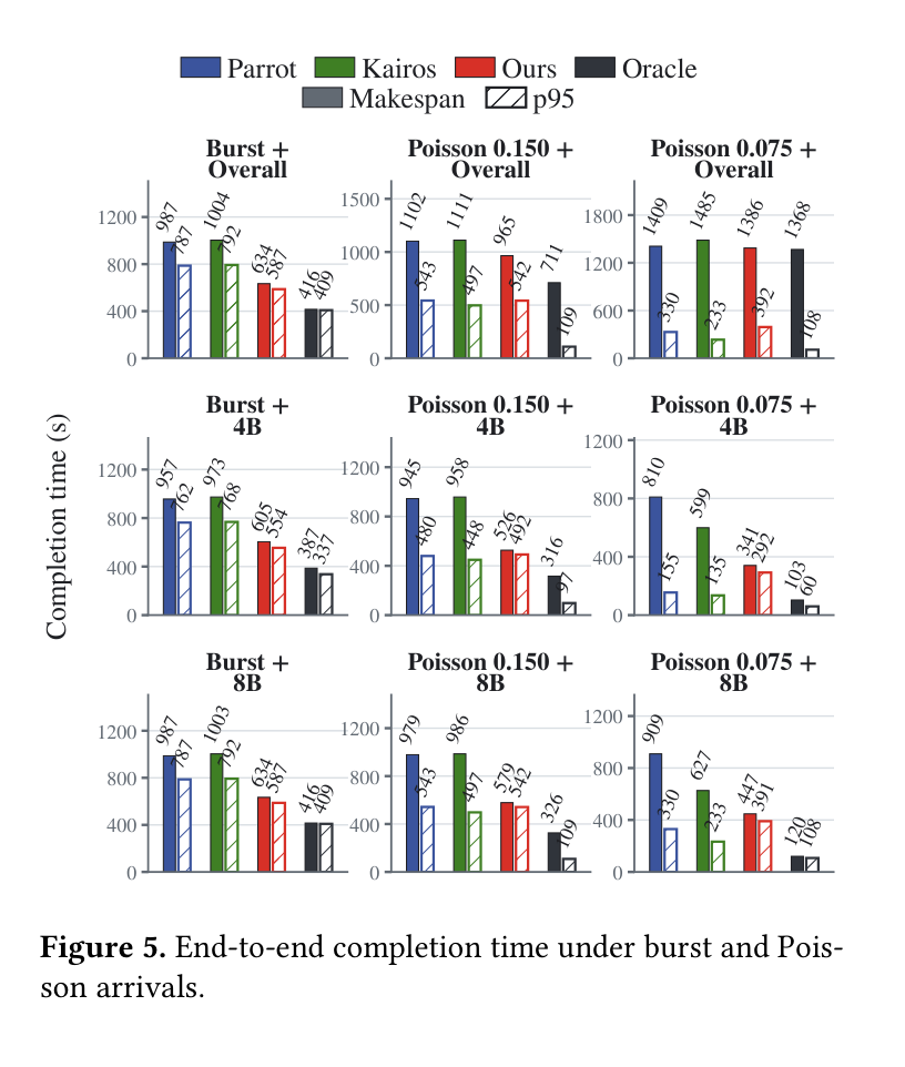
*Paper's Figure 5 (caption: "End-to-end completion time under burst and

Poisson arrivals.").* Under burst the system (Ours) dominates on makespan

(634 vs 987/1004) and p95 (587 vs 787/792), approaching Oracle (416/409).

Reader should notice the honest loss under dispersed Poisson: e.g.

Poisson 0.075 Overall p95 is 392 for Ours vs 233 for Kairos — the global

drain objective trades a local tail.



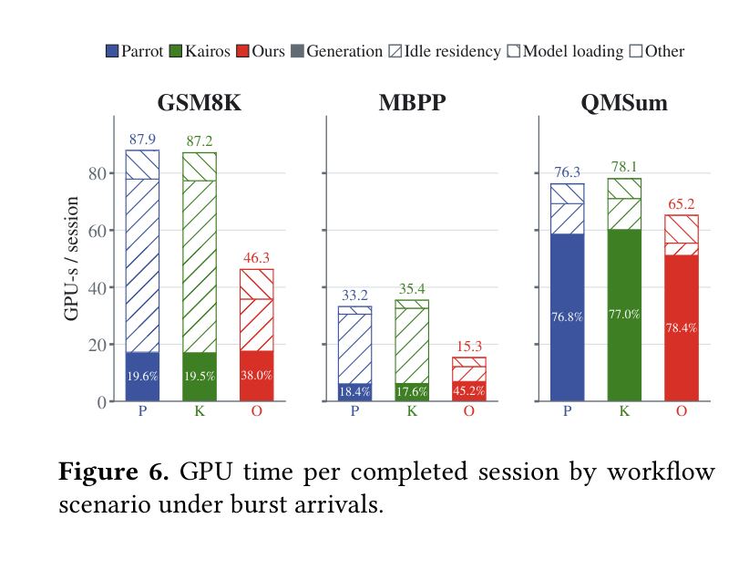
*Paper's Figure 6 (caption: "GPU time per completed session by workflow

scenario under burst arrivals.").* The stacked bars show the gain is almost

entirely from the idle-residency segment collapsing (GSM8K 60.3→18.3,

MBPP ~25→5.25, QMSum ~10.8→4.31 GPU-s), confirming the mechanism is better

model-lifecycle management rather than faster generation.



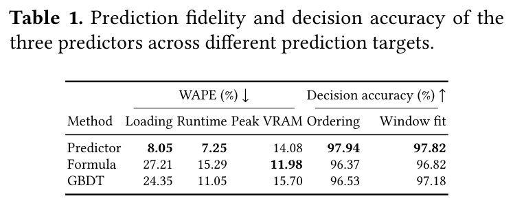
*Paper's Table 1 (caption: "Prediction fidelity and decision accuracy of the

three predictors across different prediction targets.").* Reproduced:

Method	WAPE Loading ↓	WAPE Runtime ↓	WAPE Peak VRAM ↓	Ordering acc. ↑	Window-fit acc. ↑
Predictor	8.05	7.25	14.08	97.94	97.82
Formula	27.21	15.29	11.98	96.37	96.82
GBDT	24.35	11.05	15.70	96.53	97.18

Predictor wins loading (−70.4%/−66.9%) and runtime WAPE and both decision

metrics, but the static Formula predictor wins peak-VRAM WAPE — a candid

result showing the learned model is not uniformly better.



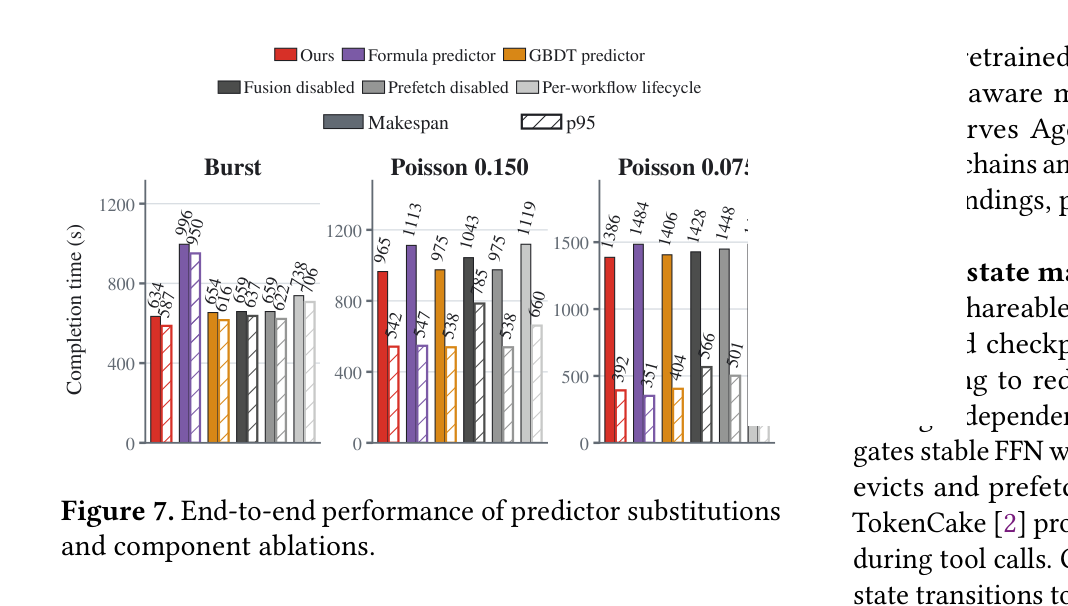
*Paper's Figure 7 (caption: "End-to-end performance of predictor

substitutions and component ablations.").* The decisive ablation:

per-workflow lifecycle (no cross-workflow coalescing) costs +7.1–16.4%

makespan — the largest makespan hit — while disabling fusion costs

+8.5–44.9% p95 (largest tail hit). Cross-workflow lifecycle coordination,

the least-emphasized mechanism, is the dominant makespan lever.

6. 论证链 #

#	Step	Support (paper-internal)
1	Under request-only scheduling, model availability (not compute) dominates waiting and GPU time.	Fig 1: 77.3–85.5% of waiting is availability delay; loading > generation GPU time.
2	Same-model node boundaries force repeated physical admission, producing a large p95 tail.	Fig 2: 39–42% of p95 session is boundary re-acquire (97.1–155.1 s).
3	Workflow progress exposes near-ready structure, so lifecycle and unit boundaries can be prepared before readiness without changing semantics.	§2.3 opportunity; §3.2 window $\mathcal{W}_t$ and physical realization $G^p_t$.
4	Accurate per-(model,request,device) prediction is required to rank devices and check feasibility online.	Eq 1–2; Table 1 shows 8.05%/7.25% WAPE and >97% decision accuracy.
5	Fusion + cross-workflow lifecycle coalescing + joint cumulative-memory scheduling reduce makespan and GPU time.	Eqs 3–12, Algorithm 1; Fig 5 (−36.8% makespan), Fig 6 (−24.63 GPU-s).
6	Removing any component degrades performance, with cross-workflow lifecycle the top makespan lever and fusion the top tail lever.	Fig 7 ablations: per-workflow +7.1–16.4% makespan; no-fusion +8.5–44.9% p95.

7. 实现 cross-reference #

[实现未公开] — the paper's footnote states "Code and data will be

released upon acceptance," so no file:line citations are available.

Reconstruction anchors for a future implementation, from the paper:

• 核心技术壁垒 (elaborated): the hardest-to-replicate piece is the online

Propagate step (Algorithm 1 line 14) that serializes co-located

operations and validates Eqs 9–11 cumulatively per transition boundary

$\tau$. Getting the memory feasibility right requires modeling transient

overlap (old weights + retained KV + engine buffers + incoming state

coexisting during a load) — a steady-state check is insufficient and will

produce OOMs that the adaptive $\rho_\kappa(t)$ term only patches after the

fact.

• 关键实现细节 (easy-to-miss tricks):
• Two different output buckets for one unit: timing uses the smallest

bucket covering the 90th-percentile observed output length of recent

same-node completions (optimistic), while admission always uses the

configured output limit (pessimistic). Using one bucket for both

silently breaks either latency accuracy or feasibility.

• Fusion admits max context but predicts summed runtime (Eq 4): the

admission envelope is $\max_i I_i$ over the chain (worst-case), yet the

release estimate is $\sum_i \widehat{T}^{\text{run}}$; conflating these

over-reserves memory or under-predicts release.

Closest open references (engine substrate only): vLLM 0.10.2 continuous

batching, on which all systems including the baselines Parrot and Kairos run.