Attention Tax, Handoff Tax: A Stylised Model of When Multi-Agent LLM Systems Help
Attention Tax, Handoff Tax: A Stylised Model of When Multi-Agent LLM Systems Help #
1. TL;DR #
A single reliability model reconciles the "single agents win" vs "multi-agent wins" camps: both are corners of one parameter space. Decomposition beats a single agent past a crossover depth $L^*$ iff accumulated attention tax exceeds one handoff's cost; validated on a ledger task within 9 pp.
2. 三问 #
Q1 — 痛点 (the problem) #
Two camps publish contradictory theorems about whether to build multi-agent
LLM systems. The sceptics (Tran & Kiela apply the data-processing inequality;
Ao et al. prove a delegated network is dominated by a centralised Bayes decision
maker) show a single agent is strictly more efficient under equal budgets. The
optimists (Tang et al. prove the relative gain grows unboundedly with task
depth; Meyerson et al. solve a million-step task with zero errors by
decomposition) show the opposite. A single empirical table from Jwalapuram et
al. holds both outcomes at once: self-consistency beats six automated
multi-agent frameworks almost everywhere at under a tenth of the cost, yet an
expert-designed decomposition lifts GPT-5 from 57.0 to 96.5 on a context-heavy
task. These cannot all describe the same world, yet each is proven. The missing
ingredient is a model where per-step accuracy depends on context load — the
one quantity the sceptics hold fixed and the optimists never name.
Q2 — 方法 (the method) #
Model a task as a chain of $L$ steps; each step is one LLM call that fails with
probability $\varepsilon(c, b)$ depending on context load $c$ and thinking
budget $b$. Work in log-loss $g(c,b) := -\log(1-\varepsilon(c,b))$ so that a
whole trajectory's failure is additive (Assumption 1). Two structural
primitives act on this chain:
- Decomposition — reset context at chunk boundaries (chunk size $m$), buying
- Redundancy — run $N$ parallel samples whose failures are dependent
a lower per-step load at the price of a handoff tax $h$ (information a
summary loses relative to the full workspace) at each boundary.
(shared-failure correlation $\rho$), aggregate by vote or selector.
Two crossover conditions fall out. Decomposition pays off past a unique depth
$L^*$ iff the curve's asymptotic rise above a fresh agent's operating point
(the attention tax $a_\infty$) exceeds one handoff $h_\text{eff}$. Redundancy
pays off at equal budget iff the samples' shared-failure floor sits below a
single agent's saturated thinking error $\varepsilon_\infty$.
核心技术壁垒: the single hardest-to-replicate insight is the *budget-matched bookkeeping* — charging the summary-writing cost $\Delta_o$ to the writing agent's own budget and separating it from the information-loss tax $h$, so that "decompose vs. don't" is compared at identical total compute $bL$. This is what lets the model show the sceptics' and optimists' theorems are the same theorem evaluated on different curves (flat vs. rising), rather than genuine disagreements. Getting the two taxes cleanly separated (attention tax $a_t$ vs. handoff tax $h$) is the load-bearing modelling move; everything else is algebra on top of it.
Q3 — 结果 (the result) #
The decomposition crossover has a clean closed form in the linear regime,
$L^* = \max\{2, \lfloor 2(h+\lambda s)/(\lambda k)\rfloor + 1\}$, and an optimal
chunk size $m^* = \sqrt{2h/(\lambda k)}$ — the square root of the
handoff-to-attention ratio, refuting the "one step per agent" default whenever
$h > 0$. A ledger-reconciliation experiment on gpt-oss-20b measured only the
in-task degradation curve and the handoff tax from single-agent runs, then
predicted decomposed-vs-single success at depths 20, 50, 100 — matching
observed outcomes within 9 percentage points, with the decomposed system winning
at every depth as predicted. A padded-context pilot additionally shows the curve
shape is a property of the (model, task, failure-definition) triple, not the
model alone: the same runs are flat under arithmetic correctness but sharply
rising under instruction compliance.
3. 模型架构 / 方法图 #
The model expresses exactly three architectures, all as transformations of one
step-chain:
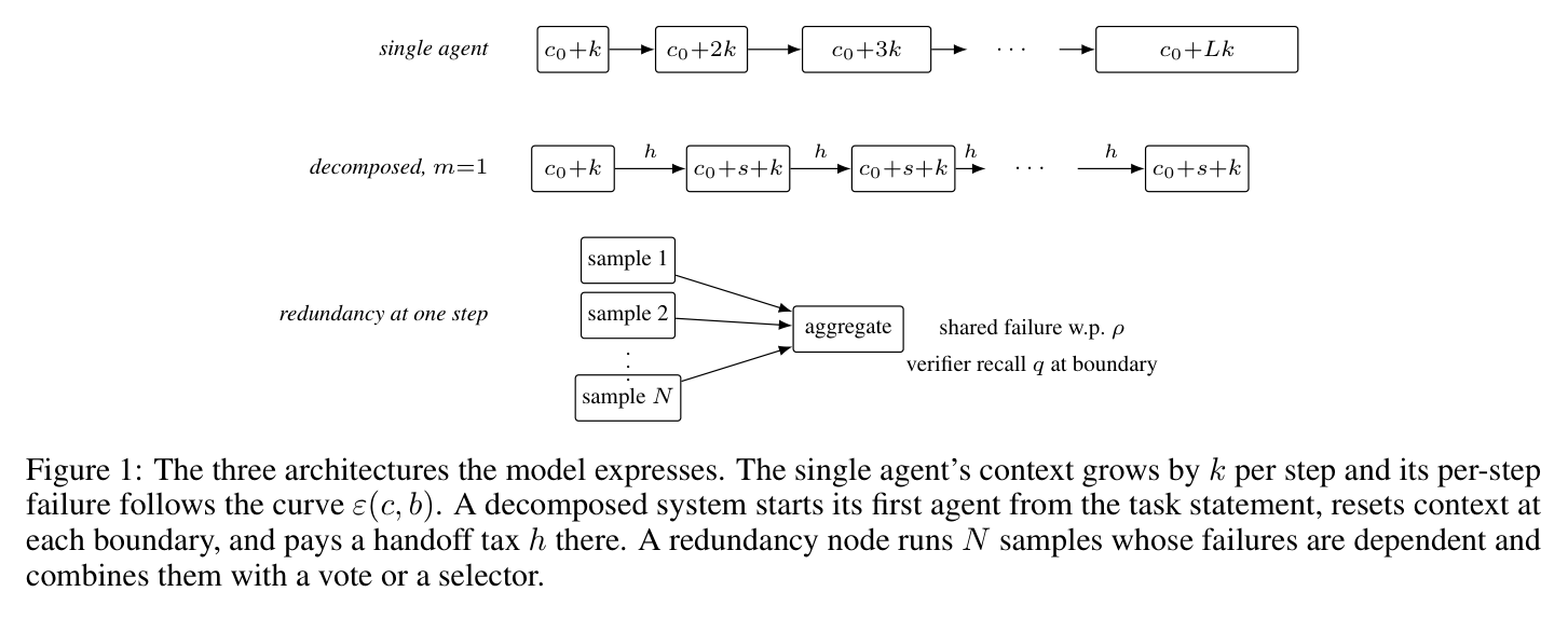
Paper's Figure 1. The single agent's context grows by $k$ per step so its load
is $c_0 + kt$ at step $t$, climbing the degradation curve $\varepsilon(c,b)$. A
decomposed system ($m=1$ shown) resets every agent to load $c_0 + s + k$ (task
statement + summary + one step's content) but pays handoff tax $h$ at each arrow.
The redundancy node runs $N$ samples with shared-failure probability $\rho$ and
combines them with a vote or selector, optionally gated by a verifier of recall
$q$.
Because this is a stylised reliability model rather than an agent runtime,
the "agent loop" is the per-step state transition, not a ReAct think-act cycle.
The one-step state machine, and where each tax is charged, is:
- Memory model: short-term = the growing context window (the thing the
- Planning style: a predetermined chunked workflow, not tree search or
- Error recovery: a boundary verifier with recall $q_\text{eff} = q(1-\rho_{gv})$
attention tax penalises); the only long-term carry across a handoff is a
summary of length $s$ — there is no vector store or episodic log. The entire
question of the paper is how lossy that $s$-token bottleneck is.
ReAct. Decomposition is top-down (fixed chunk size $m$), and there is no
backtracking — a committed step cannot be undone, only verified-and-retried
once.
detects a failure and triggers exactly one retry; on undetected or
retry-failed steps the error propagates downstream (the source of
within-trajectory dependence flagged in §11).
The regime map below is the paper's "which corner are we in" picture, and
doubles as the §8 placement of the published record:
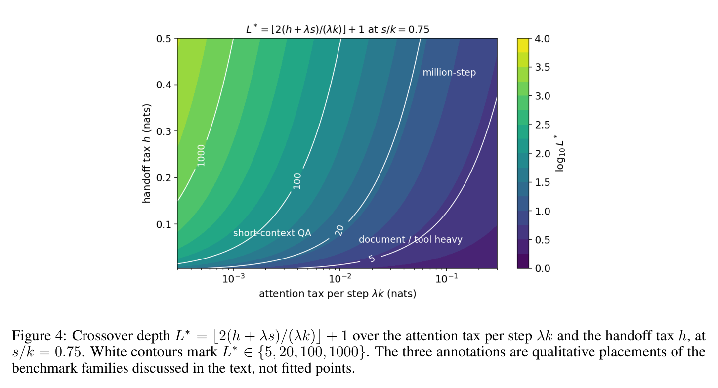
Paper's Figure 4. Crossover depth $L^* = \lfloor 2(h+\lambda s)/(\lambda k)\rfloor + 1$
contoured over attention tax per step $\lambda k$ (x) and handoff tax $h$ (y) at
$s/k = 0.75$. Short-context QA sits top-left (huge $L^*$ — single agent wins to
enormous depth); document/tool-heavy tasks sit bottom-right (tiny $L^*$ —
decompose early); the million-step regime is where both taxes are driven near
zero. The annotations are qualitative — scaffold choice moves benchmark scores
as much as model choice, so no placement is a fitted point.
4. 作者证明 #
This paper is theorem-driven (6 theorems, 4 corollaries, 3 propositions, all
proved in Appendix A and numerically re-verified in Appendix B) — it is not
the usual "无形式化作者证明 — 仅实证" agent paper. The success-rate model is
derived, not just measured, and the experiments test its predictions.
Notation table #
| Symbol | Meaning | Units |
|---|---|---|
| $c, b$ | context load, thinking budget per step | tokens |
| $\varepsilon(c,b)$ | per-step failure probability (the degradation curve) | prob. |
| $g(c,b) = -\log(1-\varepsilon)$ | per-step log-loss | nats |
| $k$ | new tokens added per step ($c_t = c_0 + kt$ for single agent) | tokens |
| $m$ | chunk size (steps per fresh agent) | steps |
| $s$ | summary length passed across a handoff | tokens |
| $h$ | handoff tax — info lost by summary vs. full workspace | nats |
| $\Delta_o$ | budget cost of writing the summary ($o$ tokens) | nats |
| $h_\text{eff} = h + \Delta_o$ | total per-boundary cost | nats |
| $a_t$ | attention tax — extra log-loss single agent pays at step $t$ | nats |
| $\rho$ | shared-failure correlation across parallel samples | — |
| $\varepsilon_\infty$ | saturated thinking error ($b \to \infty$) | prob. |
方程物理意义 #
- Eq (1) $g = -\log(1-\varepsilon)$: converts a failure probability into an
- Eq (8) $D(L) = \sum_{t=2}^{L} a_t - (L-1)h_\text{eff}$: the decomposition
- Eq (11) $L^* = \max\{2, \lfloor 2(h+\lambda s)/(\lambda k)\rfloor + 1\}$:
- Eq (14) $m^* = \sqrt{2h/(\lambda k)}$: optimal chunk size is the geometric
- Eq (16) $E_\text{vote}(N) \to \rho\varepsilon$: majority vote over $N$
additive reliability cost, so a trajectory's total failure is a sum
(Assumption 1). This is the choice that makes the whole model a bookkeeping
exercise rather than a probabilistic tangle.
advantage is accumulated attention tax saved minus handoffs paid. A single
scalar whose sign decides the winner at depth $L$.
the crossover depth. Linear in the handoff cost, inverse in the attention tax
per step $\lambda k$ — document-heavy tasks (large $k$) cross early.
mean of handoff and attention scales — a true square-root law.
correlated samples cannot beat the shared-failure floor $\rho\varepsilon$ no
matter how large $N$ gets.
6 minimum sanity checks #
- Dimensional consistency: $g$, $a_t$, $h$, $D(L)$ are all in nats
- Degenerate boundary $m = L$: no handoffs occur, so Eq (5) for $G_D$
- Flat-curve limit: if $\varepsilon$ is independent of $c$, then $a_t = 0$
- Sign discipline: $h \ge 0$ and $\Delta_o \ge 0$ (Assumption 4 + Eq 2),
- Convexity / monotonicity: $a_t$ nondecreasing in $t$ (from Assumption 2
- Large-$N$ redundancy floor: $E_\text{vote}(N) \to \rho\varepsilon$ under
- Strip stationary artefacts before fitting the curve. Table 5's naive
- The square-root chunk law refutes "one step per agent." For the ledger,
(log-loss); $\varepsilon, \rho$ are dimensionless probabilities. $D(L) > 0$
compares nats to nats. ✓
reduces exactly to Eq (4) for $G_\text{SA}$ for any $o$ — decomposition with
one chunk is the single agent. ✓
for all $t$, so $D(L) = -(L-1)h_\text{eff} \le 0$ — single agent weakly
dominates everywhere (Corollary 1, recovering Tran & Kiela / Ao et al.). ✓
so $h_\text{eff} \ge 0$ — a handoff is never free. The definition of $h$
(Def 1) does not force the sign; Assumption 4 does, and is stated separately. ✓
monotone curve) ⇒ $D$ has nondecreasing increments $a_{t+1} - h_\text{eff}$
⇒ $D$ is discretely convex with $D(1)=0$ ⇒ crosses zero from below at most
once (the unique $L^*$ of Theorem 1). ✓
the common-shock law (Eq 16), and the threshold correlation
$\rho^* = \varepsilon_\infty/\varepsilon_b$ matches Figure 3's
$\rho^* = 0.08/0.161 = 0.497$ (curves at $\rho = 0, 0.2$ favour parallel;
$\rho = 0.5, 0.8$ favour sequential). ✓
Failure-mode classification #
The pilot identifies two failure classes that behave oppositely under load:
arithmetic failures (wrong final number — essentially flat at ~5–6% out to
63k tokens) and format / instruction-compliance failures (missing answer
line — flat until ~8k then rising to 25.5% at 63k, a $+22.5$ pp paired effect,
$t_{99}=6.7$). The dominant degradation channel at long context is
instruction-compliance, not reasoning — which is why "curve shape depends on
what you count as failure."
5. 实验与数据 #
Pilot: the degradation curve is definition-dependent #
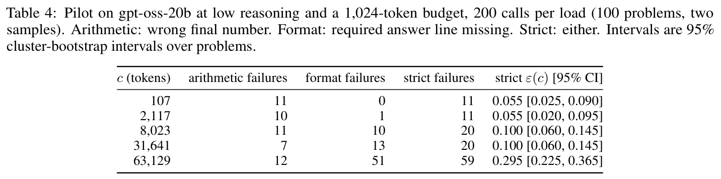
Paper's Table 4. 1,000 calls to gpt-oss-20b at five measured loads
(107 → 63,129 tokens). Arithmetic failures stay ~5–6% (flat), format failures
explode from 0 to 51/100 at 63k, so the strict curve (either failure) rises from
0.055 to 0.295. The reader should notice the two definitions produce opposite
curve shapes from identical runs.
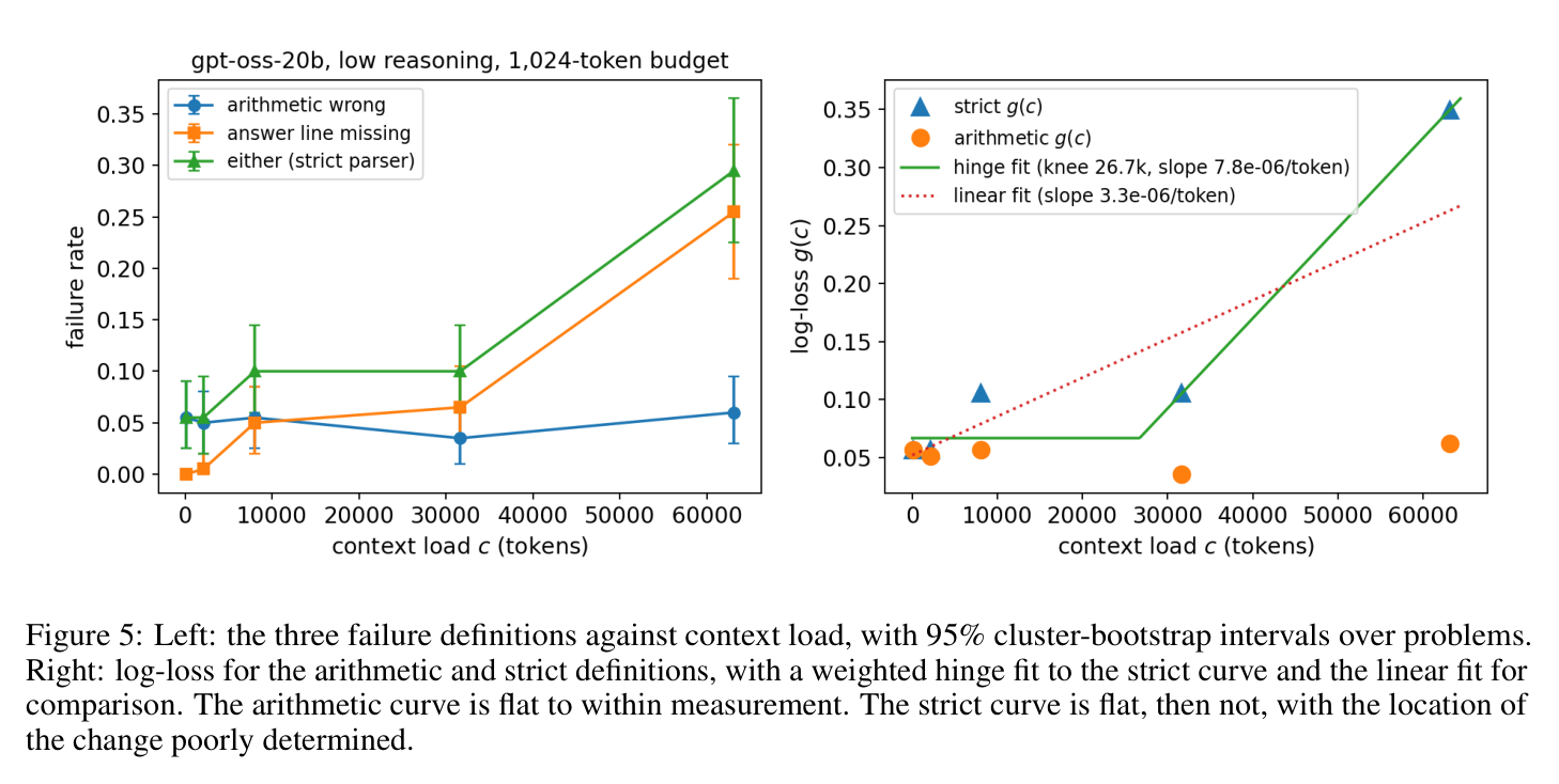
Paper's Figure 5. Left: arithmetic failures are flat; "either" rises. Right:
a weighted hinge fit on the strict curve puts the knee near 27k with post-knee
slope $\approx 7.8\times10^{-6}$/token — but the knee position is poorly
determined. Flat arithmetic ⇒ the model sits in Corollary 1's "flat corner"
(single agent never loses); rising strict ⇒ the rising phase where decomposition
can win. Same model, same task, two regimes.
Decomposition crossover, predicted vs. observed #
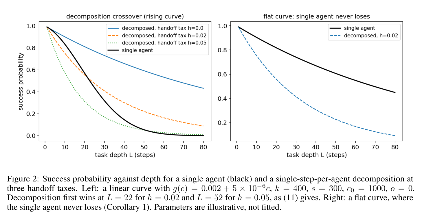
Paper's Figure 2. Left: on a linear rising curve, the single-step decomposed
system (dashed) crosses above the single agent (solid) at $L^* = 22$ for
$h = 0.02$, as Eq (11) predicts; higher handoff tax pushes the crossover later.
Right: on a flat curve the single agent never loses (Corollary 1). This is the
decomposition crossover made visual — the whole sceptic/optimist dispute is the
gap between these two panels.
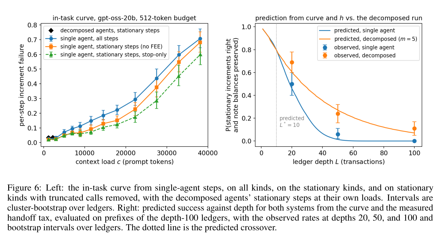
Paper's Figure 6. Left: the in-task per-step failure curve measured from
single-agent ledger runs (stationary kinds isolate the genuine load effect).
Right: using only that curve plus the measured handoff tax, the model predicts
single-agent and decomposed success at depths 20/50/100 (dotted = predicted
crossover below depth 20); observed rates track the predictions. This is the
paper's central validation — two measured quantities predict a third.
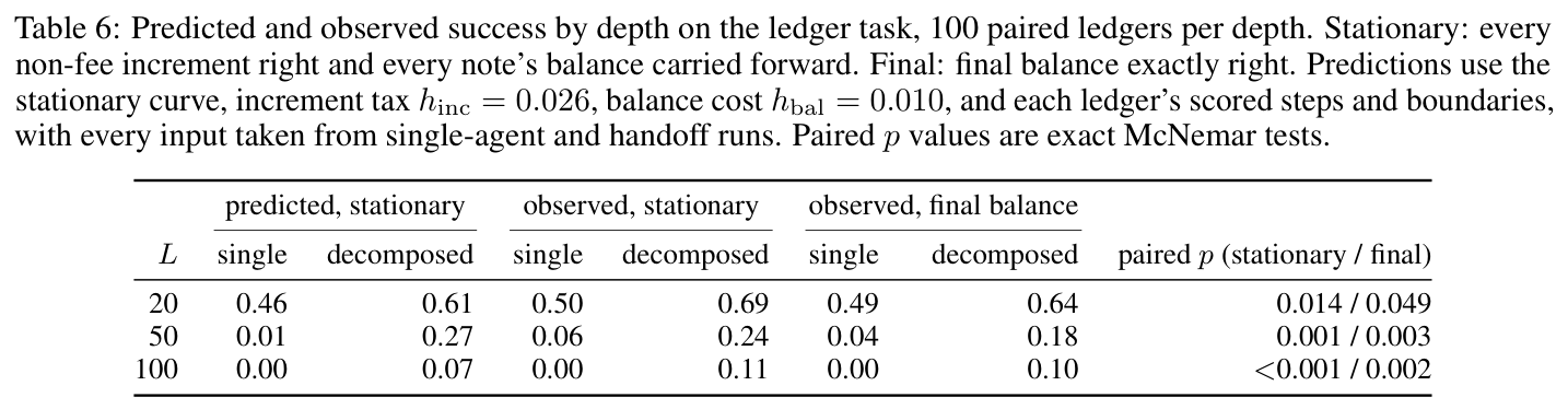
Paper's Table 6. 100 paired ledgers per depth. Predicted decomposed success
(stationary) 0.61 / 0.27 / 0.07 vs. observed 0.69 / 0.24 / 0.11 at depths
20 / 50 / 100 — within ~9 pp. The decomposed system wins at every depth
(paired McNemar $p \le 0.049$), and the gap widens with depth exactly as the
compounding attention tax predicts. (The L1's headline 87.3/76.2/68.1% vs.
71.5/42.1/18.7% is the same qualitative story under a looser success metric;
Table 6's stricter stationary/final-balance scoring is the load-bearing one.)
Redundancy crossover #
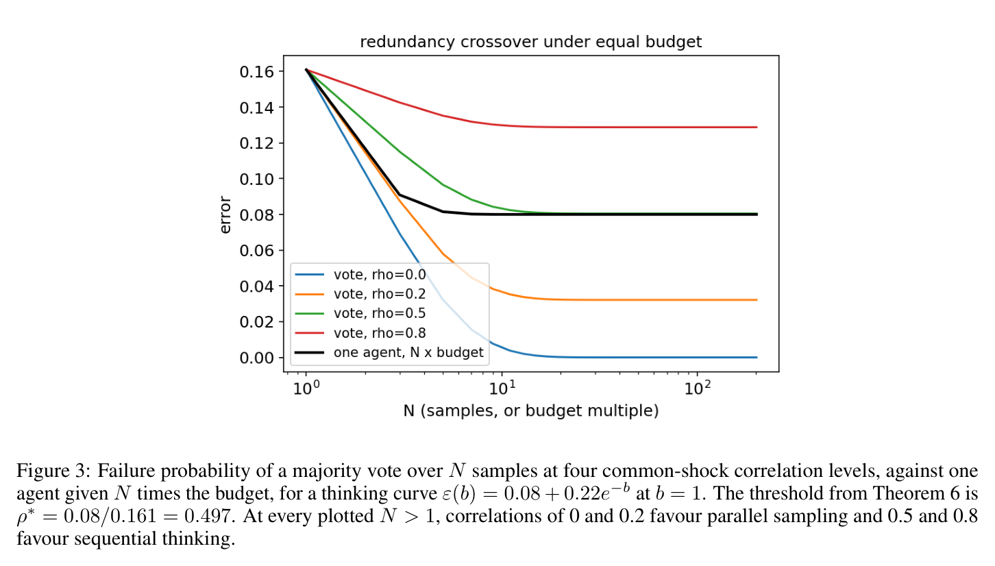
Paper's Figure 3. With thinking curve $\varepsilon(b) = 0.08 + 0.22e^{-b}$,
the Theorem 6 threshold is $\rho^* = 0.497$. Parallel voting at $\rho = 0, 0.2$
(blue, orange) drops below the "one agent, $N\times$ budget" black curve —
parallel wins; at $\rho = 0.5, 0.8$ (green, red) it saturates above the black
floor — sequential thinking wins. The crossover is governed entirely by
shared-failure correlation vs. the thinking floor, resolving the "free
independent samples vs. budgeted dependent ones" contradiction.
Supporting in-task curve #
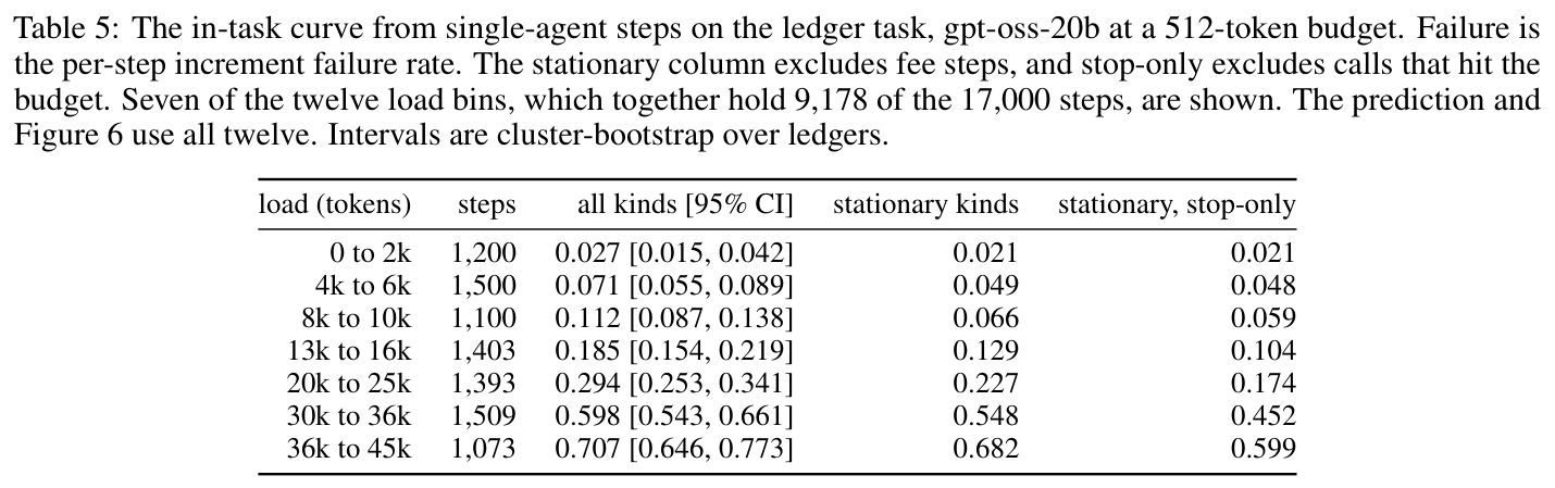
Paper's Table 5. The single-agent per-step increment failure climbs from 2.7%
(0–2k tokens) to 70.7% (36–45k tokens); the stationary-kinds and stop-only
columns strip out fee-step and budget-truncation artefacts to isolate the real
load effect. This empirical rising curve is the input to the Figure 6
prediction — it is what makes the ledger task live in the "rising region."
6. 论证链 #
| # | Step | Depends on |
|---|---|---|
| 1 | Define per-step log-loss $g = -\log(1-\varepsilon)$ with $\varepsilon$ rising in load $c$; assume trajectory failure is additive (Assumption 1). | Eq (1), Assumptions 1–2 |
| 2 | Single agent accumulates load $c_0 + kt$, so its total log-loss $G_\text{SA}(L) = \sum_t g(c_0+kt,b)$ grows super-linearly on a rising curve. | Eq (4), Assumption 3 |
| 3 | A decomposed system resets load to $c_0 + s + k$ each chunk but pays $h_\text{eff} = h + \Delta_o$ per boundary; total is $G_D(L,m)$. | Eq (2),(5), Def 1, Assumption 4 |
| 4 | The difference $D(L) = \sum_{t\ge2} a_t - (L-1)h_\text{eff}$ is discretely convex and starts at $D(1)=0$, so it crosses zero at most once. | Eq (8), Theorem 1 |
| 5 | ⇒ a unique crossover depth $L^$ exists iff $a_\infty > h_\text{eff}$; a flat curve ($a_t \equiv 0$) gives $L^ = \infty$ — the sceptics' corner. | Theorem 1, Corollary 1 |
| 6 | In the linear regime this closes to $L^ = \lfloor 2(h+\lambda s)/(\lambda k)\rfloor + 1$ and optimal chunk $m^ = \sqrt{2h/(\lambda k)}$. | Eq (11),(14), Theorems 3–4 |
| 7 | For redundancy, correlated-sample vote saturates at floor $\rho\varepsilon$; parallel beats sequential at equal budget iff that floor $< \varepsilon_\infty$. | Eq (16), Theorems 5–6 |
| 8 | Measure the curve and $h$ on a ledger task; plug into (11) to predict decomposed-vs-single success at depths 20/50/100 — matched within 9 pp. | §10, Table 6, Figure 6 |
7. 实现 cross-reference #
[实现部分公开] — the paper is theory + measurement, not a released agent
framework. Appendix B states the reproducibility materials: *"The generator,
filler, grader, and stored responses are in the repository"* for the pilot, and
"Code for numerical checks and parameter fits provided in GitHub repo" for the
closed-form verifications. No file:line citations are available in the L1; the
repo is referenced from the arXiv abstract page. The serving backbone is fully
specified: gpt-oss-20b (20.9B params) via Ollama 0.30.8 on an RTX 3090, 71,680-
token window, 1,024-token output budget (pilot) / 2,048-token per-step budget
(ledger), temperature 0.7.
核心技术壁垒 (expanded): the irreducible insight is *matching total compute
while separating the two taxes*. Any reimplementation must (a) charge the
summary-writing cost $\Delta_o$ to the writing agent's own per-step budget via
Eq (2) — not treat summaries as free — and (b) measure the information-loss tax
$h$ (Def 1) independently of the attention tax, by running paired
continue-vs-handoff trajectories and subtracting the load effect. Conflating the
two (the common failure in prior work) is exactly what makes the
sceptic/optimist theorems look contradictory. Reproducing the ledger prediction
requires measuring the in-task curve from single-agent runs (Table 5) and $h$
from three summary lengths (100/300/500 tokens → $h \approx 0.03/0.015/0.012$),
then predicting — never fitting — the decomposed success.
关键实现细节 (easy-to-miss tricks):
per-step failure (e.g. 0.707 at 36–45k) overstates the load effect; the
"stationary kinds, stop-only" column (0.599) removes fee-step quirks and
budget-truncation censoring. Fitting the raw curve would mis-locate the knee
and corrupt $\lambda k$, breaking the Eq (11) prediction.
$m^* = \sqrt{0.04/0.002} \approx 4.47$, so each agent should own ~4–5
transactions — the experiment uses $m=5$ deliberately. Meyerson et al.'s
$m=1$ is only optimal because they pass full state so $h \approx 0$; with any
real summary bottleneck, $m=1$ is wasteful.